`Limit cycle initialization`

Module: tutorials.02_EP_tissue.03B_study_prep_init.run

Section author: Fernando Campos <fernando.campos@kcl.ac.uk>

This tutorial demonstrates how to initialize a cardiac tissue with state variables obtained from a single-cell stimulation.

Conceptual Overview

Similar to in-vitro experiments, cardiac tissue is usually stabilized by pacing it at basic cycle length (BCL) in order to reduce beat-to-beat changes. However, stabilization might require a few hundred beats which can take days or even weeks to complete in organ-scale models. Unlike tissue simulations, pacing an isolated cell until it achieves its stable cycle limit is computationally feasible. In order to save computational efforts, the single-cell model state variables ( $V_{\mathrm m}$ , channel gating variables, etc.) at the end of the pacing protocol can be stored and used to initialize a tissue model. This initialization procedure is equivalent to pacing the entire tissue model in a space-clamped mode. Although this procedure is computationally cheap, it is biologically unrealistic since it ignores any differences due to the activation sequence of a previous beat. If information on the activation sequence in the cardiac tissue is available before hand, it can be used in combination with the single-cell initialization method to overcome this limitation.

Problem Setup

This example will run a simulation using a 2D sheet model (1 cm x 1 cm) in which all cells are initialized with single-cell model states stored in file INIT.sv. The file contains initial conditions of all ordinary differential equations (ODEs) describing channel gating and ionic concentrations in the chosen cellular model. The initial conditions are obtained after pacing the cell model at a prescribed BCL for a number N of beats.

Usage

To run this tutorial :

cd tutorials/03B_study_prep_init

./run.py --help 

The following optional arguments are available (default values are indicated):

--model             Model of the cellular action potential
                    Options: {MBRDR,TT2}
                    Default: Modified Beeler-Router Drouhard-Roberge (MBRDR) model
--init-method       Method to initialize the tissue model
                    Options: {none, sv_init or prepace}
                    Default: none
--bcl               Basic cycle length for repetitive single-cell stimulation
                    Default: 500 ms (2 Hz) 
--npls              Number of pulses applied to the single-cell with the given bcl
                    Default: 10

If the program is run with the --visualize option, meshalyzer will automatically load transmembrane potentials $V_{\mathrm m}$ :

./run.py --visualize

Key Parameters

The key parameter is --init-method. This will be set to one of three possible values in order to initialize the 2D sheet model:

none: all cells are initialized with the cellular model default states that are hard coded in CARP
sv_init: all cells are initialized with the cellular model states stored in file INIT.sv. Model states are computed here by running a single-cell simulation, where the cell is paced npls (default: 10 pulses) times with the prescribed bcl (default: 500ms). Model states are taken at the end of the simulation protocol.
prepace: unlike in the sv_init initialization method, where state variables are saved into a file at a prescribed time instant (usually at the end of a single-cell pacing protocol), in the prepace method cells are initialized with model states taken at different time instants depending on their a priori known activation time. The difference between the two methods is illustrated below:

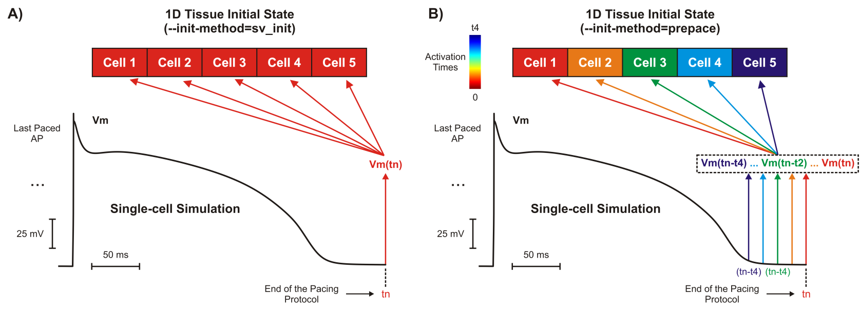
../../_images/03B_study_prep_init_sv_init_vs_prepace.png

Fig. 70 Tissue initialization methods. A) A 1D tissue model with all cells initialized with the same $V_{\mathrm m}$ as well as other model state variables (not shown) taken at the end of the single-cell simulation. B) The same 1D tissue as in A) but cells are initialized with $V_{\mathrm m}$ and other state variables (not shown) taken at different time instants. The time instants are determined based on the activation sequence know before hand: cell 1 activates at 0, cell 2 at t1, …, and finally cell 5 at time t4.

Interpreting Results

The difference between the results produced with each initialization option (i.e.: none, sv_init and prepace) can be appreciated by looking at the spatial distribution of $V_{\mathrm m}$ at time t = 0 with meshalyzer (--visualize):

../../_images/03B_study_prep_init_Vm.png

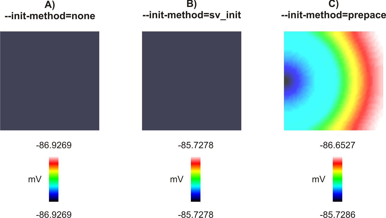
Fig. 71 Spatial distribution of $V_{\mathrm m}$ at the beggining of the simulation (t = 0 ms). A) All cells in the tissue are initialized with default model states of the MBRDR cell model. B) All cells in the tissue are initialized with the same model states in file INIT.sv. the same model states in file INIT.sv. C) Cells in the tissue are initialized with model states taken at different time instants depending on their a priori known activation time.

A) By default (--init-method=none), $V_{\mathrm m}$ at t = 0 ms will be -86.9269 mV for all cells in the tissue. This is because -86.9269 is the default initial condition of $V_{\mathrm m}$ in the MBRDR model (the initial condition of $V_{\mathrm m}$ in the TT2 is -86.2).
B) By running with the --init-method=sv_init option, $V_{\mathrm m}$ at t = 0 ms will be -85.7278 mV for all cells in the tissue. This is because -85.7278 is the initial condition of $V_{\mathrm m}$ in file INIT.sv, all model states were obtained after pacing the MBRDR model for 10 times with a bcl of 500 ms.
C) By running with the --init-method=prepace option, $V_{\mathrm m}$ at t = 0 ms will vary between -85.7286 mV (left lower corner) and -85.6527 mV (right upper corner). This is because, unlike the previous methods where all cells are initialized with the same cellular model states, cells are initialized according with model states obtained at different time instants (see above) according to the activation sequence in file LATs.dat:

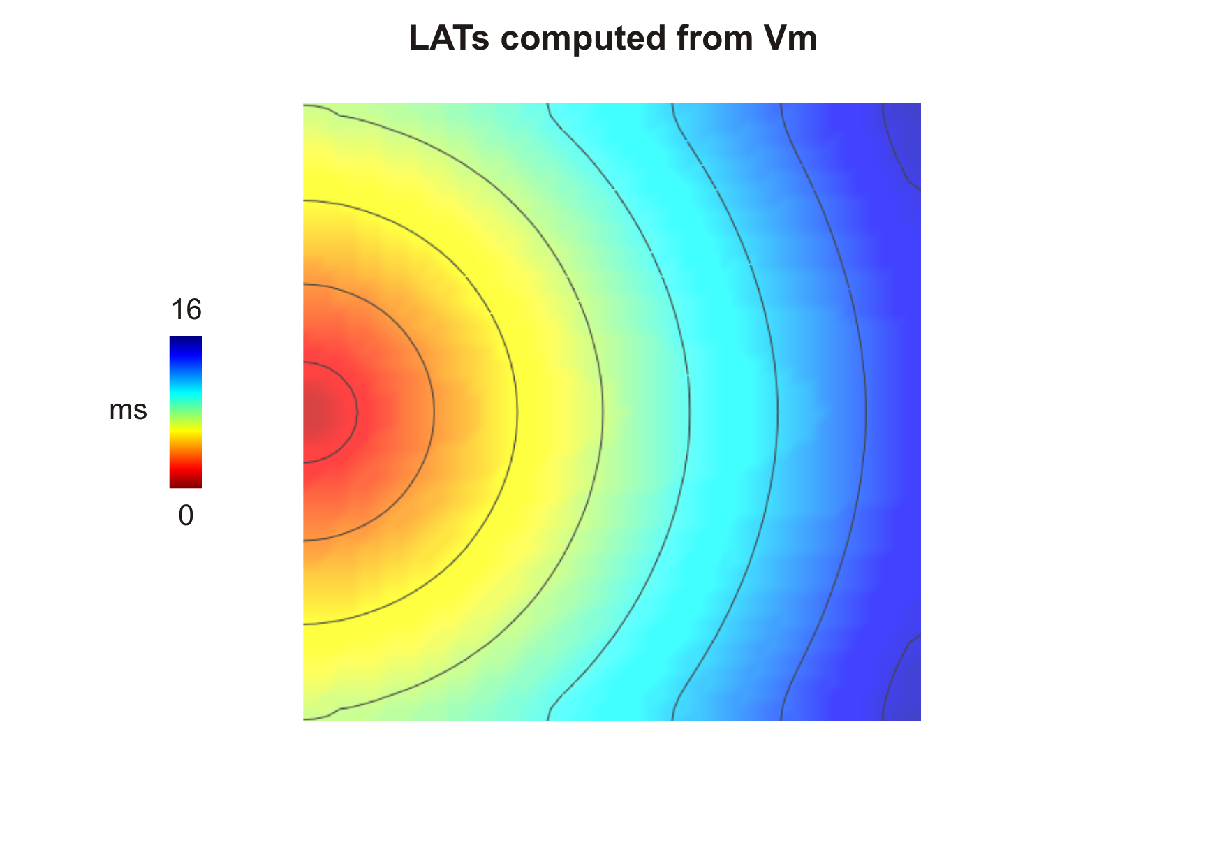
../../_images/03B_study_prep_init_prepace_LATs.png

Fig. 72 Activation sequence used to prepace the cells in the tissue.

Although the differences in $V_{\mathrm m}$ between the three initialization methods seem negligible, they can be substantial in other state variables of the ionic model with a slower time decay such as the intracellular calcium $Ca_{\mathrm i}$ . $Ca_{\mathrm i} = 0.30$ if --init-method=none and $Ca_{\mathrm i} = 0.172023$ (see file INIT.sv) if --init-method=sv_init with the bcl = 500 ms and npls = 10. These differences increase for all state variables as the bcl is reduced.

CARPentry Parameters

The relevant parameters used in the tissue-scale simulation are shown below:

# Model of the cellular action potential
-imp_region[0].im = model

# Used by the sv_init method
-imp_region[0].im_sv_init = 'INIT.sv'

# Used by the prepace method
-prepacing_beats = 10
-prepacing_lats  = 'LATs.dat'
-prepacing_bcl   = 500

imp_region[] is used to assign a model of cellular action potential to all cells in the tissue. If the sv_init initialization method is choosen, then the tissue will be initialized with cellular model states in file INIT.sv. However, if the prepace method is choosen, then the cell model in imp_region[] will be paced npls times with the given bcl. Tissue activation times in file LATs.dat are used to guide state set-up for prepacing.

Once the initial conditions are prescribed, the tissue simulation is started. In this example, a transmembrane current of 100 uA/cm^2 is applied for a period of 1 ms to the cells located at the middle of the left side of the tissue.