Concept: regions vs. gradients

Conceptual overview

1. Region-wise assignment of electrophysiological properties

   In any particular finite element mesh, each element is part of a region defined by its tag (see defining regions). When cell- or tissue-scale properties are assigned on a region-wise basis, the property in question is assigned homogeneously to all nodes and elements that belong to that region.

   One very important thing to note is that finite element nodes along the boundary between two different element regions will be assigned by carpentry to being in one region or the other. The system responsible for deciding which boundary nodes belong to which regions is predictible but not necessarily intuitive. When using region-based tagging, it is important to remain mindful of the consequences of this process. Detailed information is available in the tutorial on Cellular Dynamics Heterogeneity.

2. Gradient-wise assignment of electrophysiological properties

   As an alternative to the above-described approach, sometimes it is useful or relevant to assign properties on a node-wise basis. For example, the value of an ion channel conductance at various points across the myocardial wall might vary linearly between two values as a function of distance from the epicardium to the endocardium. This approach utilizes the carpentry adjustments interface (see adjustments) and is well-suited for defining smooth variations in electrophysiological properties. Tagging is a poor option for this type of problem, since it might require a large number of tags OR different tag-wise division for gradients in different properties (e.g., a transmural gradient in one conductance and an apicobasal gradient in another).

Problem Setup

This example will run two simulations using a 2D sheet model (1 cm x 1 cm) in which GKr and GKs values are smaller at the bottom of the sheet (y = 0) and larger at the top of the sheet (y = 1 cm). In the first simulation, the domain will be subdivided into four regions, each one with a distinct scalar multiplier for GKr and GKs:

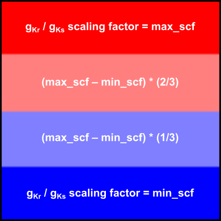
Fig. 76 Region-wise assignment of properties. Tissue is subdivided into four regions each of which is assigned different properties.

In the second simulation, the domain will consist of one unified region but the GKr and GKs values will be scaled continuously (via linear gradient) from the bottom to the top:

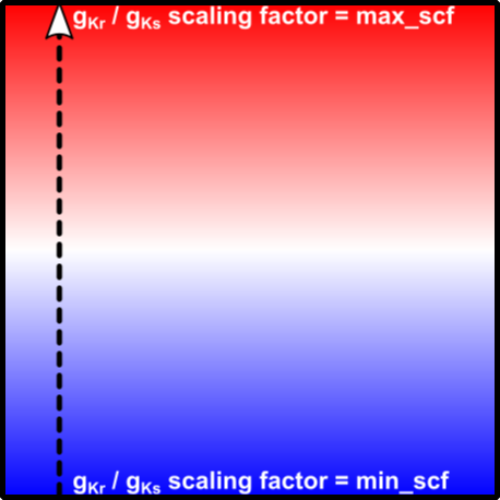
Fig. 77 Gradient-wise assignment of properties. There is only one tissue region and GKr/GKs values vary continuously from low (bottom) to high (top).

Usage

The following optional arguments are available (default values are indicated):

./run.py --min_scf     = 0.1      # lower bound scaling factor (min = 0.000, max = 0.999)
         --max_scf     = 2.0      # upper bound scaling factor (min = 1.000, max = 10.00)

If the program is run with the --visualize option, meshalyzer will automatically load a map showing the difference in action potential durations between the two simulations:

./run.py --visualize

Interpreting Results

With the default parameters, the program will perform the two simulations as described above. When the vm.igb files are visualized, it will be apparent that the depolarisation patterns are approximately the same but the repolarisation sequences are markedly different due to the variable representations of GKr/GKs heterogeneity. The side-by-side animation shown here is for the vm sequences produced by the test using the default parameters:

Fig. 78 Comparision of membrane voltage over time () for Region-wise (left) and Gradient-wise (right) variability in GKr/GKs.

The program will also produce APD.dat files in the relevant simulation subdirectories, which can also be visualized in meshalyzer to appreciate the exact distributions of APD:

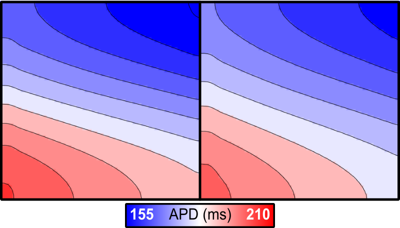
Fig. 79 Comparision of action potential duration for Region-wise (left) and Gradient-wise (right) variability in GKr/GKs.

Notably, although the effect on repolarisation is definitely more pronounced than that on depolarisation, the resulting differences in APD are subtle, as shown by the maps that can be seen using the –visualize function:

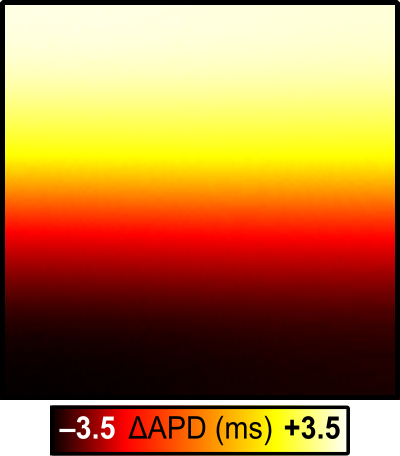
Fig. 80 Difference in action potential duration (APD) between region-based and gradient based repolarisation heterogeneity