Conductive heterogeneity (gregion)
Module: tutorials.02_EP_tissue.05B_Conductive_Heterogeneity.run
Section author: Patrick Boyle <pmjboyle@gmail.com>
This tutorial details how to assign different conductivities to different parts of a simulated tissue slice using region-wise tagging.
Problem Setup
This example will run one simulations using a 2D sheet model (1 cm x 1 cm) that has been divided into four regions (striped horizontally from top to bottom, each occupying 1/4 of the total mesh). Test parameters can be modified to explore the consequences of setting conductivity different values, adjusting anisotropy ratio (i.e., longitudinal:transverse), adjusting whether the different regions are electrically coupled to each other or isolated, and choose the electrical stimulus type.
Usage
The following optional arguments are available (default values are indicated):
./run.py --reg0_giL          = 2.00000  # conductivity along fibre direction (i.e., :math:`\sigma_{iL}`) in region 0 (bottom slice)
         --reg1_giL          = 0.50000  # as above, but for second region
         --reg2_giL          = 0.12500  # as above, but for third region
         --reg3_giL          = 0.03125  # as above, but for fourth region
         --anisotropy_factor = 4        # factor by which transverse conductivities are smaller than longitudinal (i.e., :math:`\sigma_{iL}`::math:`\sigma_{iT}` = [factor]:1)
         --split             = 0        # flag that can be asserted to electrically isolate regions instead of having them coupled to each other
         --non_planar_stim   = 0        # flag that can be asserted to use one point stimuli in each region instead of a planar stimulus
If the program is run with the --visualize option, meshalyzer will automatically
load a map showing the activation sequence in response to electrical stimulation.
./run.py --visualize
Interpreting Results
By default, the activation sequence in response to simulation will be as below:
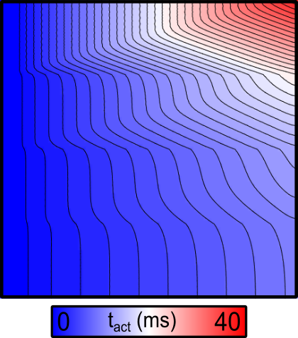
Fig. 81 2D map of activation times ( ) in response to stimulation at the
left-hand side of the sheet with default parameters. Note the delayed activation
in the top part of the sheet.
) in response to stimulation at the
left-hand side of the sheet with default parameters. Note the delayed activation
in the top part of the sheet.
There are several noteworthy observations:
- As expected, the conduction velocity in the bottom region (which has the highest conductivity value assigned) is faster than in the regions above.
- Since the stimulus is applied to the left-hand side of the sheet, the resulting wavefronts in each region are all approximately planar. As such, the effect of tissue anisotropy is relatively minimal in this example.
- The conduction velocity (CV) values in the different regions can be (very roughly) approximated by taking the activation times along the righthand side of the sheet and dividing the width of the mesh (1 cm) by those values:
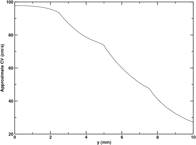
Fig. 82 Graph of approximate conduction velocity (CV) as a function of distance along the y-axis, from bottom to top. See text for details.
To get a better idea of the exact relationship between conductivity values and CV, re-run
the example with the --split option:
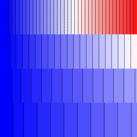
Fig. 83 Activation sequence produced by asserting the --split flag. The different regions
are now electrically de-coupled from each other.
Now that the individual regions are electrically isolated from each other, we can observe the “native” relationship between conductivity and CV. Here, we see that the approximate CV values in the four regions are, from top to bottom:
- 0: 102.7 cm/s (
 = 2.00000 mS/mm)
 - 1: 77.7 cm/s ( = 0.50000 mS/mm)
- 2: 47.5 cm/s ( = 0.12500 mS/mm)
- 3: 25.6 cm/s ( = 0.03125 mS/mm)
Since the conductivity values in adjacent regions are separated by a factor of 4, this
serves as a reminder that the approximation 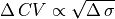 ,
derived from the linear core conductor model of bioelectric propagation, does not generally
hold up very well in the context of mondomain simulations of cardiac tissue.
,
derived from the linear core conductor model of bioelectric propagation, does not generally
hold up very well in the context of mondomain simulations of cardiac tissue.
Finally, to get a ckear idea of how the anisotropy ratio affects the properties of impulse
propagation, re-run the example with the --non_planar_stim option:
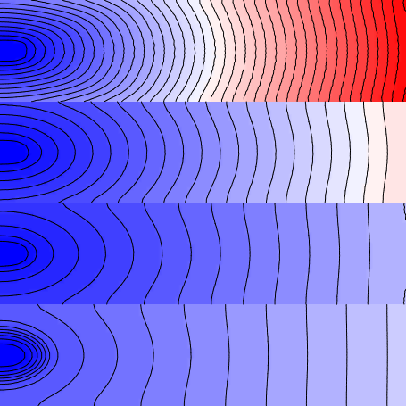
Fig. 84 Activation sequence produced by asserting the --non_planar_stim flag. There is now
a discrete point stimulus in each region instead of one big planar stimulus.
Note that wavefronts now emanate from four point sources along the left-hand side of the sheet and the activation isolines are clearly ellipsoidal, with propagation in the Y-axis direction slower than that in the X-axis direction. This behaviour arises from the fact that the fibre orientations in this sheet are uniformly from left to right (i.e., all entries in the .lon file are <1 0 0>.
This example highlights the effect of reduced transverse conductivity ( ),
in this case by a factor of 4. The
),
in this case by a factor of 4. The --anisotropy_factor argument can be adjusted to
explore the effect of different magnitudes of adjustment.
One final interesting observation from the last simulation discussed above, note that although the CV in the bottom-most stripe is the fastest of the four regions (as expected), the wavefront actually arrives at the right side of the sheet later than for the stripe above. This is because the source-sink dynamics at the stimulation site vary between regions. In this case, we observe that the dramatically increased coupling in the bottom-most stripe mean that excitation dissipates more quickly from the stimulus site (i.e., the tissue is more “sink-ey”, meaning that we are closer to the critical threshold below which the stimulus will not elicit a propagating response.
What’s Going On Under The Hood?
The relevant part of the .par file for this example is shown below:
#############################################################
num_gregions             = 4
#############################################################
gregion[0].g_il          = 2.0
gregion[0].g_it          = 2.0
gregion[0].g_in          = 2.0
gregion[0].num_IDs       = 1
gregion[0].ID[0]         = 0

gregion[1].g_il          = 0.5
gregion[1].g_it          = 0.5
gregion[1].g_in          = 0.5
gregion[1].num_IDs       = 1
gregion[1].ID[0]         = 1

gregion[2].g_il          = 0.125
gregion[2].g_it          = 0.125
gregion[2].g_in          = 0.125
gregion[2].num_IDs       = 1
gregion[2].ID[0]         = 2

gregion[3].g_il          = 0.03125
gregion[3].g_it          = 0.03125
gregion[3].g_in          = 0.03125
gregion[3].num_IDs       = 1
gregion[3].ID[0]         = 3
Each gregion[] structure contains information about a different stripe in the mesh.
The number of gregion[] entries is controlled by the num_gregions variable.
For the purposes of this exercise, the main variables changed by the command-line
arguments are the .g_il and .g_it entries, which control the conductivity values
( and , respectively) in the relevant tagged
regions. Although the fibres in this example are uniformly oriented from left to
right, this is frequently not the case in organ-scale simulations, due to the
laminar structure of cardiac tissue. In general, for each element in a region,
the “longitudinal” direction is defined by the corresponding vector entry in the
.lon file. Also note, the .g_in entries are not used except when simulations are
conducted using meshes that have two vectors defined for each element instead of
just one (i.e., longitudinal instead of transverse) – otherwise, the assumption
is that  . Example .lon file headers are shown below:
The relevant part of the .par file for this example is shown below:
# .lon file with one set of vectors
1
0.6 0.4 0
0.4 0.6 0
# ... (one line per element in .elem file)

# .lon file with one set of vectors
2
1 0 0 0 1 0
1 0 0 0 1 0
# ... (one entry per element in .elem file)