Cellular dynamics heterogeneity (imp_region)

Problem Setup

This example will run one simulation using a 2D sheet model (1 cm x 1 cm) that has been divided into four regions (striped horizontally from top to bottom, each occupying 1/4 of the total mesh). Test parameters can be modified to explore the consequences of setting different cell-scale dynamics in the four regions. Optional flags can be used to modify the stimulus type or determine whether or not the different regions are electrically coupled.

Usage

The following optional arguments are available (default values are indicated):

./run.py --help 
  --variable            { gNa OR gKs OR gKr OR gK1 OR gss OR gtof OR gtos }
                        parameter that should be tuned up (or down, if --tune_down is asserted
  --tune_down           tune selected variable down instead of up
  --split               electrically isolate regions
  --non_planar_stim     use point stimuli in each region instead of a planar stimulus
  --show_vm             visualize vm(t) instead of depolarization times

If the program is run with the --visualize option, meshalyzer will automatically load a map showing the activation sequence in response to electrical stimulation, unless the --show-vm argument is given, in which case vm(t) is shown instead. Note that asserting the latter flag also prompts the program to run a longer simulation (300 ms instead of 50 ms) so that depolarization and repolarization can both be appreciated.

Key Parameters

The first key parameter is --variable. This will be set to one of seven possible values in order to modulate one of the possible ion channel conductances in the UCLA rabbit ionic model:

• gNa: fast sodium current conductance (default)
• gKs: slow delayed rectifier potassium current conductance
• gKr: rapid delayed rectifier potassium current conductance
• gK1: inward rectifier potassium current conductance
• gss: steady-state potassium current conductance
• gtof: fast inactivating transient outward potassium current conductance
• gtos: slow inactivating transient outward potassium current conductance

The slab is subdivided into four regions. The bottom-most stripe will be simulated under control conditions. The second stripe from the bottom will be simulated with the selected --variable either increased or decreased by a factor of two; this is where the second key parameter, --tune_down, comes into play: if that flag is asserted, the conductances of the selected --variable are decreased in stripes above the bottom-most; otherwise, the values are increased:

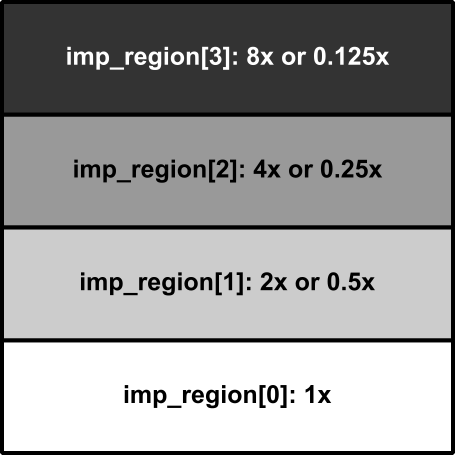
Fig. 85 Schematic showing the division of the tissue sheet into five distinct regions, each of which will have different cellular dynamics. The selected ion channel conductance is scaled UP from bottom to top by default, unless the --tune_down flag is asserted.

Examples

Example 1: Default parameters (increased gNa)

The activation sequence for the default parameters looks like this:

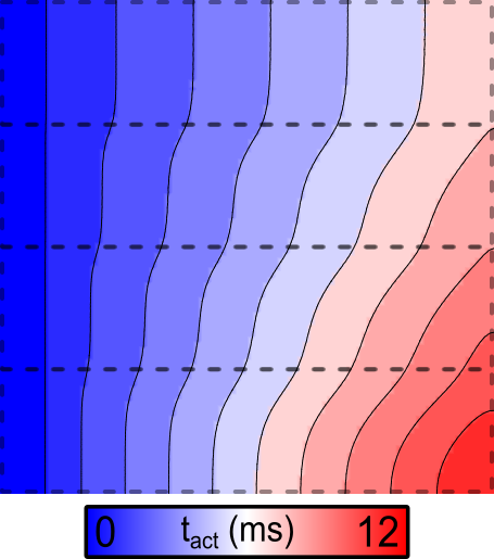
Fig. 86 Activation sequence in response to stimulation at the left side of the sheet for the default parameter set, for which fast sodium channel conductance () is scaled up from 1x at the bottom to 8x at the top.

Note the marked acceleration of conduction velocity (CV) in the upper regions, which are simulated with increased gNa.

Example 2: Decreased gNa

If the simulation above is repeated with the --tune_down flag asserted, the resulting activation sequence looks like this:

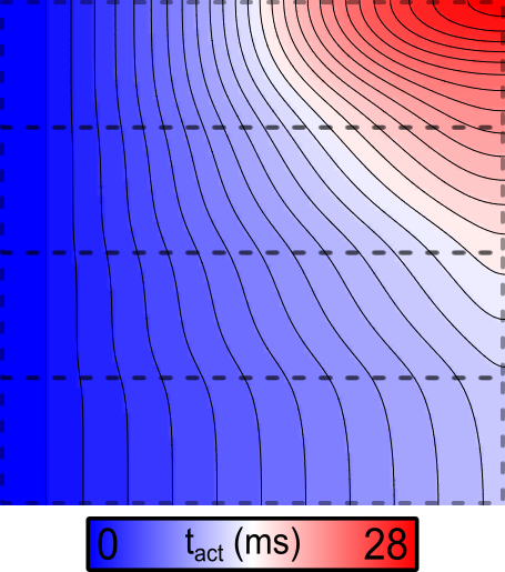
Fig. 87 Activation sequence in response to stimulation at the left side of the sheet when the --tune_down flag is asserted, so fast sodium channel conductance () is down from 1x at the bottom to 1/8 at the top.

Note that the scale bar for this figure differs from the image shown above. Here, there is dramatic CV slowing in the upper regions.

Example 3: Effect of optional parameters

If the --split and --non_planar_stim flags are asserted instead of the --tune_down flag, the following activation pattern is observed:

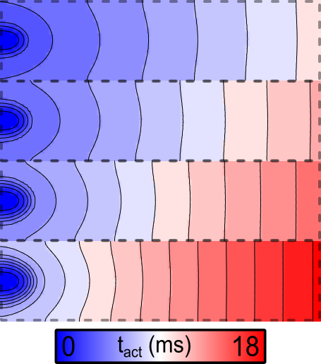
Fig. 88 Effect of asserting --split and --non_planar_stim flags. Regions are electrically separated and stimulated from point sources.

Example 4: Varying repolarizing currents

Finally, as an initial example of how the experiment can be used to explore the effects of changing repolarizing current instead of depolarizing currents, when the --variable=gKr and --show_vm arguments are given, the following excitation sequence is seen:

Fig. 89 Membrane voltage over time (), which can be visualized instaed of activation sequence, which makes it easier to observe heterogeneities in APD produced by scaling repolarizing current conductance instead of .

Note that repolarization occurs much earlier in the upper layers of the sheet in this case, due to the large increase in IKr resulting from the change in gKr.

What’s Going On Under The Hood?

The relevant part of the .par file for this example is shown below:

#############################################################
num_imp_regions          = 4
#############################################################
imp_region[0].im         = converted_UCLA_RAB
imp_region[0].num_IDs    = 1
imp_region[0].ID[0]      = 0
imp_region[0].im_param   = "gNa*1"

imp_region[1].im         = converted_UCLA_RAB
imp_region[1].num_IDs    = 1
imp_region[1].ID[0]      = 1
imp_region[1].im_param   = "gNa*2"

imp_region[2].im         = converted_UCLA_RAB
imp_region[2].num_IDs    = 1
imp_region[2].ID[0]      = 2
imp_region[2].im_param   = "gNa*4"

imp_region[3].im         = converted_UCLA_RAB
imp_region[3].num_IDs    = 1
imp_region[3].ID[0]      = 3
imp_region[3].im_param   = "gNa*8"

Each imp_region[] structure contains information about a different stripe in the mesh. The number of imp_region[] entries is controlled by the num_imp_regions variable. For the purposes of this exercise, the main variables changed by the command-line arguments are the .im_param entries, which control the ionic model parameters passed to the LIMPET interface by carp. For any particular ionic model, the list of possible paramters can be obtained by running:

bench --imp=[im name] --imp-info

Important Note

It is important to appreciate that that there is ambiguity in the determination of which nodes belong to which regions, since some nodes are found on the boundary between two or more regions:

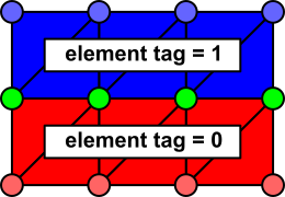
Fig. 90 Schematic illustrating ambiguity in determination of which nodes belong to which regions.

In this case, the red nodes clearly belong to whatever imp_region includes .ID[] = 1 in its list of element IDs. Likewise, the cell-wise identity of the blue nodes is clear. However, if tags 1 and 2 are assigned to different imp_region[] entries, it is unclear which entry should apply to the green nodes.

Carp resolves this ambiguity on the basis of the order of imp_region[] entries. For this case, let’s say “0” is in the tag list imp_region[X].ID and “1” is in a different tag list imp_region[Y].ID. Then, the boundary (i.e., green-colored) nodes will be assigned to the imp_region with the HIGHER index. So, if X>Y, the green nodes are assigned to imp_region[X], etc. In cases where a node is shared by elements that are assigned to multiple imp_regions, the highest imp_region[] index always “wins”. The value of the element tags themselves are NOT taken into account when assinging boundary nodes to imp_regions.

Note that this assignment process can be queried directly by loading the output file imp_region.dat in meshalyzer, which provides the imp_region[] index for each node in the mesh. To illustrate this point, consider the following .par file section as an alternative to the one shown above:

#############################################################
num_imp_regions          = 4
#############################################################
imp_region[0].im         = converted_UCLA_RAB
imp_region[0].num_IDs    = 1
imp_region[0].ID[0]      = 3
imp_region[0].im_param   = "gNa*8"

imp_region[1].im         = converted_UCLA_RAB
imp_region[1].num_IDs    = 1
imp_region[1].ID[0]      = 2
imp_region[1].im_param   = "gNa*4"

imp_region[2].im         = converted_UCLA_RAB
imp_region[2].num_IDs    = 1
imp_region[2].ID[0]      = 1
imp_region[2].im_param   = "gNa*2"

imp_region[3].im         = converted_UCLA_RAB
imp_region[3].num_IDs    = 1
imp_region[3].ID[0]      = 0
imp_region[3].im_param   = "gNa*1"

In terms of tags and properties, the same elements are assigned to groups with the same properties. The bottom stripe (i.e., tag = 0) is a region with gNa*1 but instead of being in imp_region[0] it is in imp_region[3]. As a result, all nodes along the boundary betweeen elements TAGGED 0 and 1 (i.e., the top edge of the bottom-most stripe) will be assigned to the imp_region[] with gNa*1 (i.e., ID #3). As illustrated here, similar differences will exist along the boundaries between other tagged element regions, due exclusively to the change in parameter ordering:

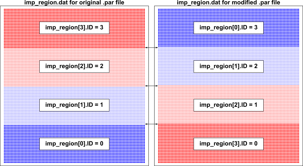
Fig. 91 Example illustrating consequences of differences in imp_region[] ordering.

It is important to understand this behavior of the simulator, since it can have major effets on the overall behaviour of simulations, especially when there are multiple tissue types with dramatically different electrophysiological properties distributed in a chaotic pattern (e.g., interdigitated regions of normal tissue, peri-infarct zone with remodeled EP, and scar with passive electrical properties).

In other words, cave seduxit astutia.