Phase singularities

Detection Algorithm

There are many different algorithms which can be used to detected filaments, which are summarised nicely in Clayton et al [1].

Locating filaments and phase singularities therefore relies on finding the lines or points of intersection of activation and recovery. This may be done explicitly or else by first transforming activation into phase. The term phase singularity refers to the fact that such a point is surrounded by tissue exhibiting all different values of phase; thus, that point itself does not have a defined phase value. In terms of activation and recovery intersection, you can think of a spiral wave core to be where the wavefront and waveback encroach on oneanother, which would be where activating tissue meets recovered (diastolic) tissue.

The method used in CARPentry relies on explicitly finding the intersection of activation and recovery. The isosurface of activation is simply found by finding the surface corresponding to a certain membrane potential level, . This is usually chosen to be around the point of activation of the sodium channel, so approximately -40mV. Note that in some complex cases of VF or when it is used to analysis simulated optical mapping signals, the action potential amplitude may well be significantly lower than during sinus rhythm, and thus this value may want to be lowered. The surface of recovery is usually defined similarly to be where , thus representing recovered and diastolic tissue. If this method is used then it is important to also define the time-window over which this is evaluated over. These two approaches are shown in the Figure below. The detection algorithm is implemented in GlFilament which can be used standalone or as a post-processing option.

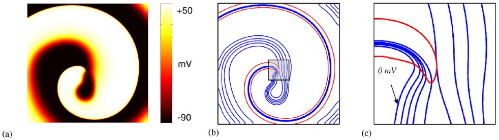
Representation of a spiral wave (a) with (b) showing isolines of voltage (blue) and recovery (red). Panel (c) shows a zoomed-in region close to the spiral core, demonstrating how the intersection of activation and recovery successfully highlight a phase singularity. Taken from Clayton et al [1]

Experimental Parameters

Phase singularity detection can be performed in either 2D or 3D with CARPentry. However, it is restricted to meshes that are triangles or tetrahedra.

The performance of the algorithm is controlled by just two experimental parameters. the isofilament threshold and the iso-filament interval. The isofilament threshold defines the value of which correlates to activation. It therefore depends on the cell model. The isofilament interval defines time window over which is evaluated. According to Clayton et al [1] for most cell models this would be 2 ms, however, longer values seem to work better for the implementation in CARPentry.

Output

The output of the filament detection is of the form of a series of Auxiliary Grid files which can be loaded into Meshalyzer for visualisation purposes. These constitute .pts_t, .elem_t files. Important to note is that these files are, by default, stored in the same location as the mesh itself. In addition a series of files called filament_*.cnnx are also produced. These represent the connections (which define the filaments, or parts of filaments), at each time-slice. Connections simply define the two node numbers which therefore represent a line in space (i.e. a line of phase singularity in this case). Note that the connections files are stored in the same place as the executable to compute the filaments was run.

Primarily, the output from the filament detection is for visualisation purposes. However, an additional series of files are also produced which list the elements that a line of phase singularity is present within. These are (currently) stored as filament_* martin.elem. These are stored in the same place as the connection files. They are very useful for looking at the connectivity of filaments in 3D i.e. deciding how many separate unique filaments you have at any given time, and looking for filament birth/death/splitting/amalgamation. More details of such further quantification of filament dynamics can be found in Bishop & Plank (2012) [2].

Visualisation

Once the data is loaded into Meshalyzer, to improve visibility, in the connection properties window the size of the connections should be increased, surfaces are turned off and data are visualized on vertices. Vertex opacity can be turned on using the threshold level used for filament detection as the threshold for opacity. If filaments were detected correctly, the connections should appear right at the isoline.

Experiments

The below defined experiment runs on re-computed voltage data due to the domain size and time required to simulate a sustained arrhythmia. To run this experiment

cd ${TUTORIALS}/02_EP_tissue/09_filaments

Run

./run.py --help

to see all exposed experimental parameters.

--iso_threshold       defines the value of :math:`V_{m}`  which approximately correlates to activation (default value is -20 mV).

--iso_intv            defines time window over which :math:`dV_{m}/dt=0` is evaluated (default value is 8 ms).

./run.py --iso_threshold -20 --iso_intv 8 --visualize