Fibre Angle Stimulation I - Rotation
Module: tutorials.02_EP_tissue.14_bidm_rotation.run
Section author: Laura Marx <laura.marx@medunigraz.at>
Introduction
The aim of this tutorial is to study the effect of fiber orientation on the electrical behavior of cardiac tissue.
Generally, electrical properties of the myocardial tissue can be described by the bidomain model
accounting for the intracellular and extracellular domain. The domains are of anisotropic nature, the intracellular domain
even more so than the extracellular domain resulting in ‘’unequal anisotropy ratios’’ affecting the heart’s electrical behavior
causing two effects ‘’rotation’’ and ‘’distribution’‘. This tutorial focuses on the ‘’rotation’’ effect, which occurs when
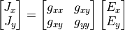
two spaces have different degrees of anisotropy. If considering an isotropic tissue the electrical field  and current density
  would point in the same direction. It follows that
  with g being
the scalar conductivity. In anisotropic tissue this is not the case as the conductiviy tensor rotates towards the fiber direction
relative to . As anisotropy ratios are unequal in the intra- and extracellular space current densities
with g being
the scalar conductivity. In anisotropic tissue this is not the case as the conductiviy tensor rotates towards the fiber direction
relative to . As anisotropy ratios are unequal in the intra- and extracellular space current densities  and
and
 are rotated by different amounts. [3]
Experimental Setup
Analytical vs. Numerical Setup:
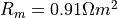
Given is a 2D strip of infinite length of width W=10mm in which fibers are oriented with  (shown as grey dotted lines in the figure below).
Conductivities are given as
(shown as grey dotted lines in the figure below).
Conductivities are given as  S/m,
S/m,  S/m,
S/m,  S/m and
  S/m
where L and T indicate directions along and transverse to the fiber orientation, respectively (Anisotropy ratios are unequal!). The
tissues membrane surface-to-volume ratio and the resistance are given as
S/m
where L and T indicate directions along and transverse to the fiber orientation, respectively (Anisotropy ratios are unequal!). The
tissues membrane surface-to-volume ratio and the resistance are given as 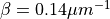 and
and
 . For numerical analysis we assume that the length L of the strip is not infinite, but
 . For the data given choosing L=60mm should suffice. The spatial resolution should be used as height of the strip (only one layer of 3D elements).
The analytical solutions should be used to verify the numerical results in 3D.
. For the data given choosing L=60mm should suffice. The spatial resolution should be used as height of the strip (only one layer of 3D elements).
The analytical solutions should be used to verify the numerical results in 3D.
Model Settings: A hexahedral FE model with dimensions of 60mm x 10mm x 1mm shall be generated functioning as cardiac tissue strip.
An orthotropic fiber setup is used with a sheet angle of  .
.
Electrical Settings:
As passive ionic model the modified Beeler-Router Druhard-Roberge model as implemented in LIMPET is used with  set to
  and .
Current is injected by Electrode A at x=-L/2 and withdrawn by electrode B at x=+L/2. Electrode C is located at x=0 and can be gounded or not.
and .
Current is injected by Electrode A at x=-L/2 and withdrawn by electrode B at x=+L/2. Electrode C is located at x=0 and can be gounded or not.
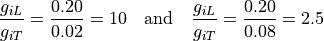
Conductivity Settings: Unequal anisotropy is assigned using the following values:
gregion[0].g_il          = 0.2
gregion[0].g_it          = 0.02
gregion[0].g_in          = 0.02
gregion[0].g_el          = 0.2
gregion[0].g_et          = 0.08
gregion[0].g_en          = 0.08
Solution Method: The simulation is solved using the parabolic formulation of the bidomain equations with the Crank-Nicolson method.
Input Parameters and Usage
Go to the following directory to run underlying experiment:
cd ${TUTORIAL}/02_EP_tissue/14_bidm_rotation/
The following experiment specific options are available (default values are indicated):
./run.py --angle                #pick fiber angle (0 is along the long edge of the preparation) (default:45)
         --resolution           #choose mesh resolution in um (default: 250)
         --grounded {on, off}   #turn on/off ground (default:off)
Note
If a high mesh resolution is chosen it may take longer to run. You may use the --np option to increase number of cores.
To visualize results with meshalyzer use --visualize.
--grounded - A ground can be used or not. In the latter case, no grounding electrode
is used, that is, a pure Neumann-problem is solved. A rank-one stabilization is used
in this case which essentially enforces the integral over the extracellular potential
to be zero at each instant in time, but no specific point is clamped.
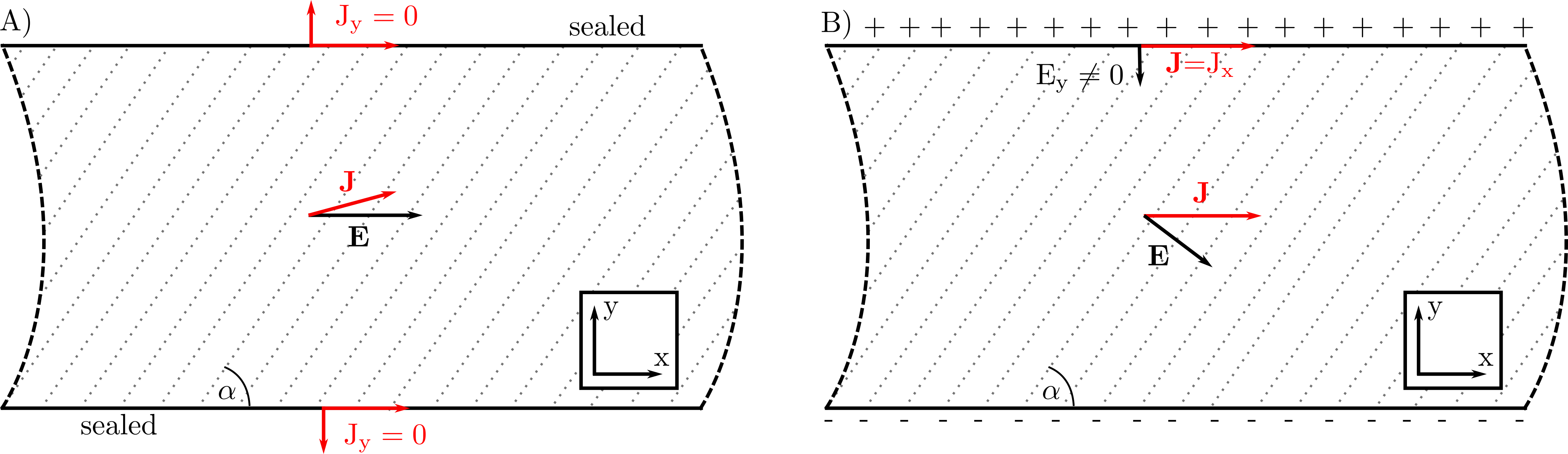
Theoretical Considerations
At  electrical current is injected into the tissue strip and the same current is withdrawn at .
Initially, an electrical field is setup at the center of the strip at y=0, which is oriented along x, but current density is oriented towards the
fiber orientation (running against a sealed boundary under angle
electrical current is injected into the tissue strip and the same current is withdrawn at .
Initially, an electrical field is setup at the center of the strip at y=0, which is oriented along x, but current density is oriented towards the
fiber orientation (running against a sealed boundary under angle  , see Fig. A) with
Since  current will be directed towards the sealed ends at
  . Due to
  charge will accumulate at the sealed ends
which sets up an electrical field (see Fig. B). From
charge will accumulate at the sealed ends
which sets up an electrical field (see Fig. B). From
and the fact that at must be zero it can be concluded that makes and angle with x given by
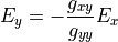
Due to  and
and  neither nor can depend on y.
Now we considering a bidomain with unequal anisotropy ratios.  and
and  must be zero individually at sealed boundaries.
Thus,
must be zero individually at sealed boundaries.
Thus,
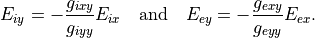
As the tissue strip is infinitely long 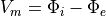 cannot be a function of x thus
and it follows that
Thus,

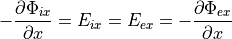
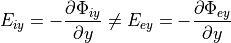
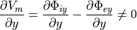
It can be concluded that there must be a y-directed gradient of  causing membrane polarisation near the boundary (see Fig. C).
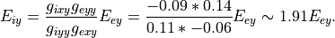
Near the center of the strip at y=0 the net current must be in direction of x with  , but due to rotation intra- and
extracellular densities and make an angle with the x-axis. Intra- and extracellular field are equal (see Fig. D):
, but due to rotation intra- and
extracellular densities and make an angle with the x-axis. Intra- and extracellular field are equal (see Fig. D):

which implies that the  vanishes near the center as

Results
Analytical Solution:
First conductivity ratios are computed as
followed by conductivity tensors in the fiber coordinate system

and in the cartesian coordinate system assuming a fiber angle of  :
:

and

At the sealed boundaries and must be zero individually at sealed boundaries thus,

As the tissue strip is infinitely long cannot be a function of x thus
and it follows that
Thus,
holds with 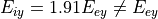 as well as
with  .
.
It can be concluded that the y-directed gradient of causes membran polarisation near the boundaries (see results of numerical solution).
Near the center of the strip at y=0 the net current must be in direction of x with , but due to rotation intra- and
extracellular densities and make an angle with the x-axis. Intra- and extracellular field are equal:
which implies that the vanishes near the center (see results of numerical solution) as

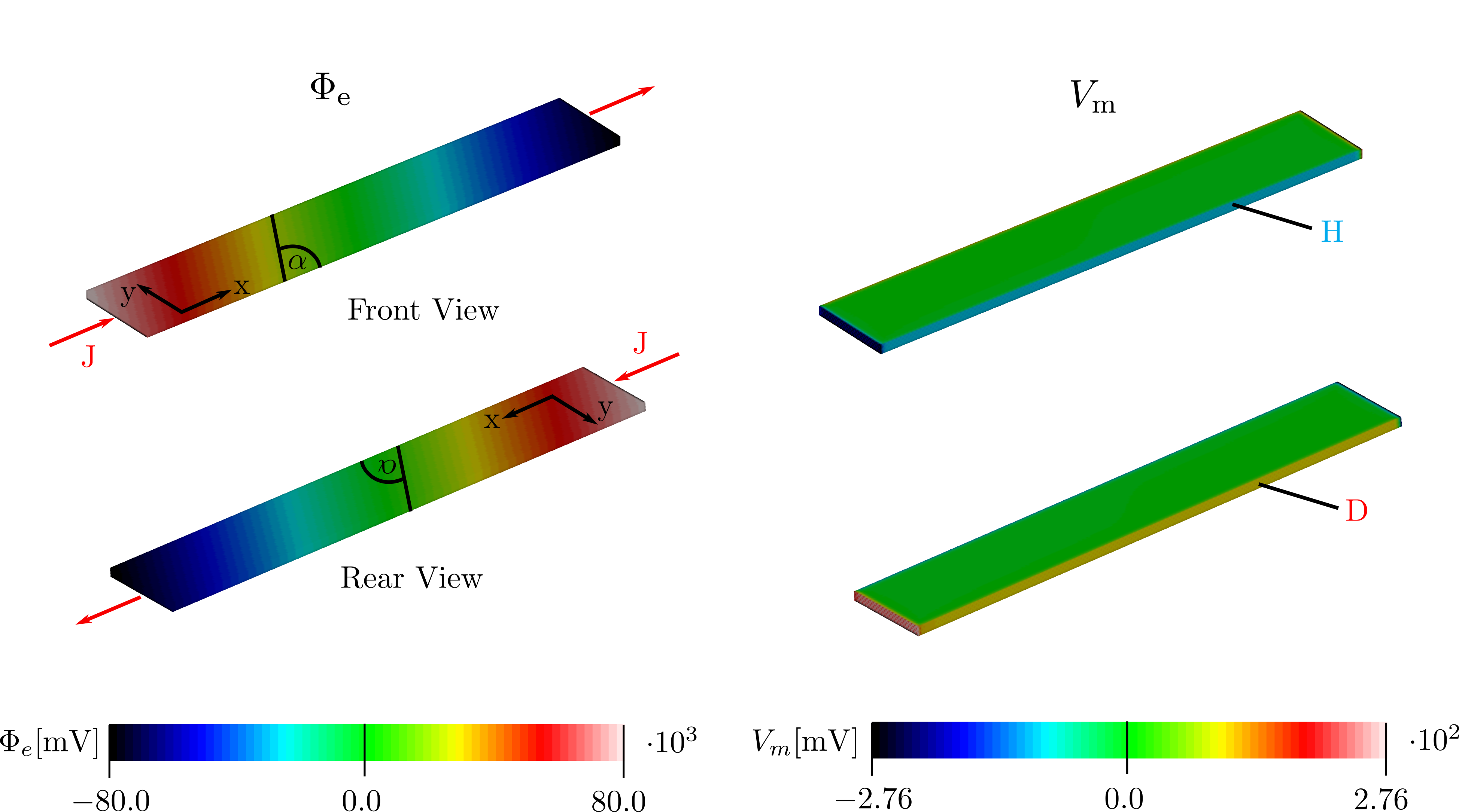
Numerical Solution: Front and rear view of simulated tissue strip for :
Interpretation
Simulation results confirm theoretical expectations. Gradient  hyperpolarizes and depolarizes edges of the tissue strip at
 and
and  and vanishes at the center of the strip.
Literature
| [1] | Sepulveda, Nestor G., Bradley J. Roth, and John P. Wikswo Jr., Current injection into a two-dimensional anisotropic bidomain, Biophysical journal 55.5 (1989): 987-999. |
| [2] | Bradley J. Roth, and Marcella C. Woods, The magnetic field associated with a plane wave front propagating through cardiac tissue, IEEE transactions on biomedical engineering, Vol. 46, No.11 (1999). |
| [3] | Bradley J. Roth, How to explain why unequal anisotropy ratios is important usind pictures but no mathematics, International Conference of the IEEE Engineering in Medicine and Biology Society (2006). |