`Fiber Angle Stimulation II - Distribution`

Module: tutorials.02_EP_tissue.15_bidm_distribution.run

Section author: Laura Marx <laura.marx@medunigraz.at>

Introduction

The aim of this tutorial is to study the effect of changes in fiber orientation on the electrical behavior of cardiac tissue. Generally, electrical properties of the myocardial tissue can be described by the bidomain model accounting for the intracellular and extracellular domain. The domains are of anisotropic nature, the intracellular domain even more so than the extracellular domain resulting in ‘’unequal anisotropy ratios’’ affecting the heart’s electrical behavior causing two effects ‘’rotation’’ and ‘’distribution’‘. This tutorial focuses on the ‘’distribution’’ effect, which refers to the relative conductivity of the intracellular and extracellular domains. As current takes the path of least resistance more current will flow in the domain where conductivity is the highest. The relative amount of current in the two spaces is defined by their respective anisotropy ratios. [3]

Experimental Setup

The setup is identical to the setup in the ‘’Fiber Angle Stimulation I - rotation’’ tutorial, except a gradual change in fiber orientation along x is implemented.

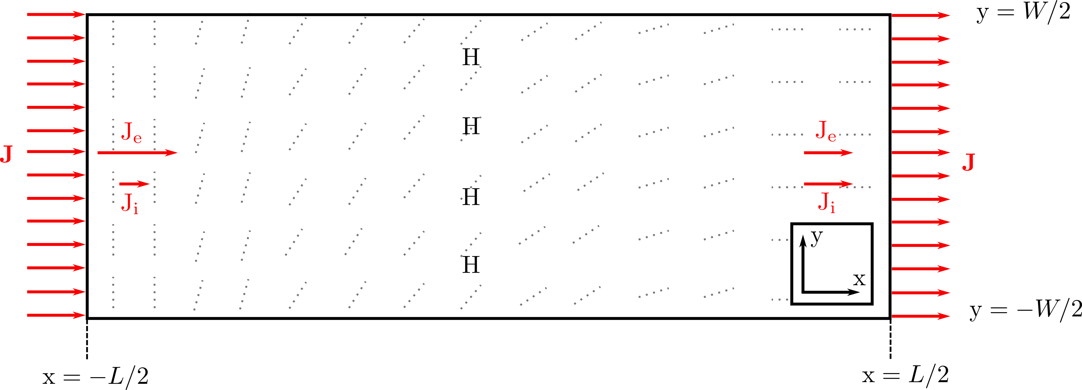
A 2D strip of infinite length of width $W=10$ mm is given. The fiber angle varies from $\alpha = 90^{\circ}$ to $\alpha = 0^{\circ}$ over the length of the strip. (marked as dotted gray lines in Fig. below). Conductivities are given as $g_{iL} = 0.2$ S/m, $g_{iT} = 0.02$ S/m, $g_{eL} = 0.2$ S/m and $g_{eT} = 0.08$ S/m where L and T indicate directions along and transverse to the fiber orientation, respectively (Anisotropy ratios are unequal!). The tissues membrane surface-to-volume ratio and the resistance are given as $\beta = 0.14\mu m^{-1}$ and $R_{m} = 0.91 \Omega m^{2}$ .

../../_images/02_EP_tissue_15_bidm_distribution_experimentalsetup.png

For numerical analysis we assume that the length L of the strip is not infinite, but $L\gg\lambda$ . For the data given choosing L=60mm should suffice. The spatial resolution should be used as height of the strip (only one layer of 3D elements). Thus, a hexahedral FE model with dimensions of 60mm x 10mm x 1mm is generated functioning as cardiac tissue strip. An orthotropic fiber setup may be used if the sheet angle differs from $0^\circ$ . As passive ionic model the modified Beeler-Router Druhard-Roberge model as implemented in LIMPET is used with $R_{m}$ set to $0.91 \Omega m^{2}$ and $\beta = 0.14\mu m^{-1}$ . Current $\mathbf{J}$ is injected by Electrode A at x=-L/2 in x-direction and withdrawn by electrode B at x=+L/2. Electrode C is located at x=0 and can be gounded or not.

Unequal anisotropy is assigned using the following values:

gregion[0].g_il          = 0.2
gregion[0].g_it          = 0.02
gregion[0].g_in          = 0.02
gregion[0].g_el          = 0.2
gregion[0].g_et          = 0.08
gregion[0].g_en          = 0.08

The simulation is solved using the parabolic formulation of the bidomain equations with the Crank-Nicolson method.

Input Parameters and Usage

Go to the following directory to run underlying experiment:

cd ${TUTORIAL}/02_EP_tissue/14_bidm_rotation/

The following experiment specific options are available (default values are indicated):

./run.py --angle-epi            #pick left bound of fiber angle (0 is along the long edge of the preparation) (default:-60)
         --angle-endo           #pick right bound of fiber angle (default:+60)
         --sheet-angle          #pick sheet-angle and thus use orthotropic fiber setup (default:0, transversely isotropic fiber setup)
         --gil                  #pick intracellular conductivity longitudenally to fiber direction (S/m) (default: 0.2)
         --git                  #pick intracellular conductivity transversely to fiber direction (S/m)  (default: 0.02)
         --gel                  #pick extracellular conductivity longitudenally to fiber direction (S/m)  (default: 0.2)
         --get                  #pick extracellular conductivity transversely to fiber direction (S/m)  (default: 0.08)
         --duration             #pick duration of simulation (ms)
         --resolution           #choose mesh resolution in um (default: 250)
         --grounded {on, off}   #turn on/off ground (default:off)

Note

If a high mesh resolution is chosen it may take longer to run. You may use the --np option to increase number of cores. To visualize results with meshalyzer use --visualize.

--grounded - A ground can be used or not. In the latter case, no grounding electrode is used, that is, a pure Neumann-problem is solved. A rank-one stabilization is used in this case which essentially enforces the integral over the extracellular potential to be zero at each instant in time, but no specific point is clamped.

Results

Numerical solutions are shown in terms of the extracellular potential $\phi_e$ and transmembran voltage $V_m$ (frontal and rear view of strip). The fiber angle is chosen to vary from $90^{\circ}$ to $0^{\circ}$ over the strip (transversely isotropic fiber setup with sheet angle of $0^\circ$ .

Interpretation

On the left side of the tissue strip (see Fig. below, hyper and depolarisation effects at sealed boundaries are ignored) fibers are oriented in y-direction and current flows perpendicular to the fibers. Extracellular conductivity transverse to fiber orientation $g_{eT}=0.08$ is much bigger than the intracellular conductivity in this direction with $g_{iT}=0.02$ . As current takes the path of least resistance more current will flow in the extracellular space. From x=-L/2 to x=+L/2 the fibers orientation changes gradually along x reaching a fiber angle of $0^\circ$ towards the end of the strip. Intra- and extracellular conductivities are equal in fiber direction with $g_{iL}=g_{eL}=0.20$ resulting in similar current densities $J_i$ and $J_e$ . In the middle of the strip, where the fiber angle varies, current must redistribute from the extracellular domain to the intracellular domain causing hyperpolarization of the tissue. [3]

../../_images/02_EP_tissue_15_bidm_distribution_analytical.png

Simulation results confirm theoretical expectations. It can be observed that $\phi_e$ is rotated towards the fiber direction over length of the strip. Gradient $\frac{\partial{V_m}}{\partial{y}}$ hyperpolarizes and depolarizes edges of the tissue strip at $y=-W/2$ and $y=+W/2$ but due to distribution effect based on changing fiber angle only around the center, where current must redistribute from the extracellular to the intracellular domain.

Literature

[1]	Sepulveda, Nestor G., Bradley J. Roth, and John P. Wikswo Jr., Current injection into a two-dimensional anisotropic bidomain, Biophysical journal 55.5 (1989): 987-999. [Pubmed] [Full]

[2]	Bradley J. Roth, and Marcella C. Woods, The magnetic field associated with a plane wave front propagating through cardiac tissue, IEEE transactions on biomedical engineering, Vol. 46, No.11 (1999). [Pubmed]

[3]	(1, 2) Bradley J. Roth, How to explain why unequal anisotropy ratios is important usind pictures but no mathematics, International Conference of the IEEE Engineering in Medicine and Biology Society (2006). [Pubmed]