Law of Laplace
Module: tutorials.04_EM_tissue.02_laplace.run
Section author: Matthias Gsell <matthias.gsell@medunigraz.at>
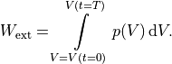
This example verifies the computed stress and the computed work using a simple spherical shell geometry and time-varying Neumann boundary condition applied on the inner boundary. To verify the computed stress, we use the law of Laplace, see [2], to estimate the wall stress and compare it against the mean computed stress. For the work varification, we compute the external work analytically and compare it against the computed internal work.
Stress Verification
To verify the stress, we use the law of Laplace to estimate the wall stress (wall tension).The
law of Laplace can be used to describe
the wall stress of a spherical shell in terms of the surface pressure applied on the inner boundary,
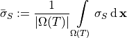
see Figure Fig. 132. To estimate the wall tension, we consider the geometry
at time  with pressure
 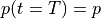 and radii
  .
.
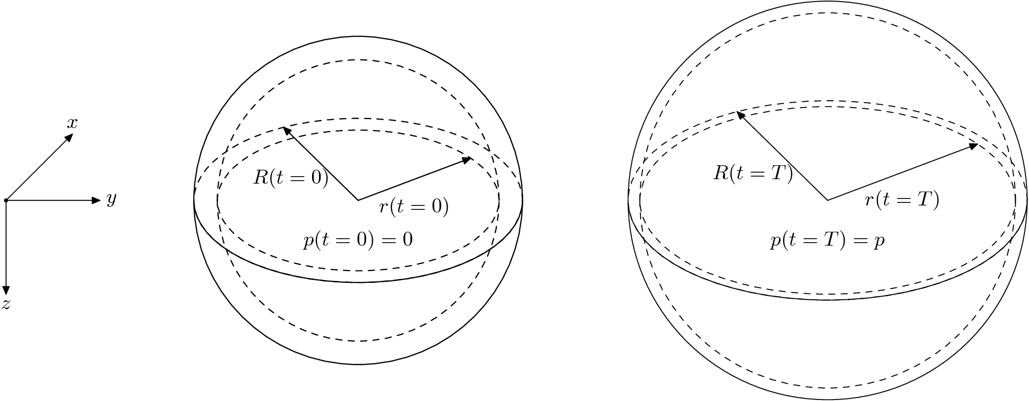
Fig. 132 Deformation at time step  and
and  .
.
Derivation Of Laplace’s Law
To derive Laplace’s law we want to use the balance of forces. We assume that the center of the spherical shell
is the origin and we denote the inner radius of the deformed geometry by  and the outer radius by
 with
with  , see figure Fig. 133.
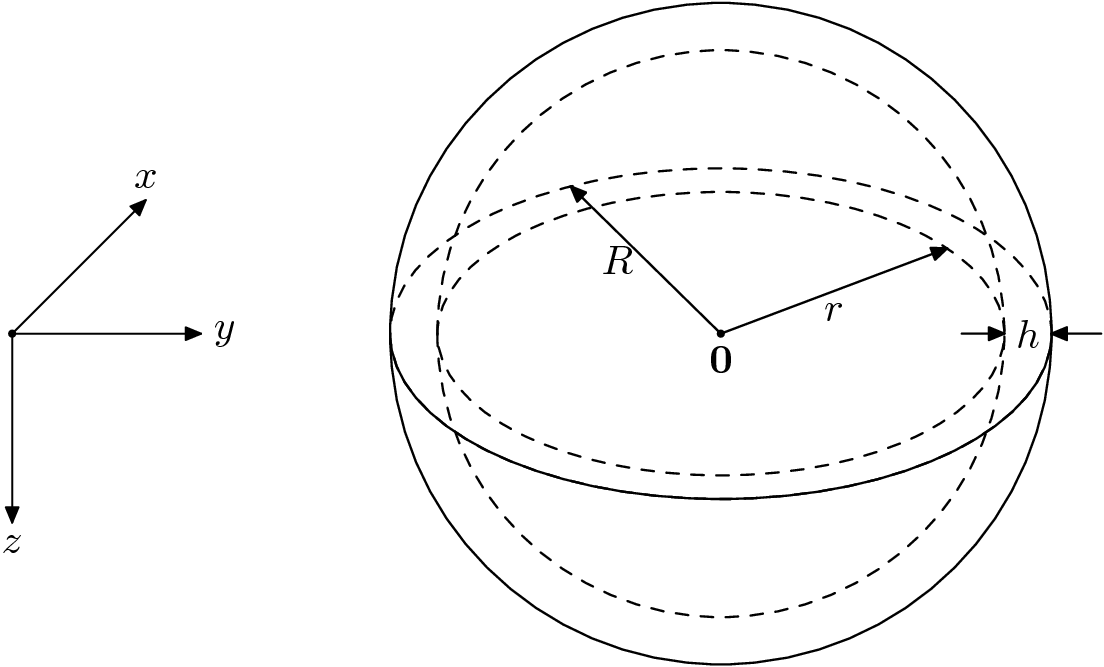
Fig. 133 Geometrical setting.
By  we denote the wall thickness which is given by
  . Next, we clip the geometry using the x-y-plane
as a clipping plane and obtain two equally sized shells, see figure Fig. 134.
. Next, we clip the geometry using the x-y-plane
as a clipping plane and obtain two equally sized shells, see figure Fig. 134.
Fig. 134 Acting forces.
The force vector acting on the inner surface is given in spherical coordinates by
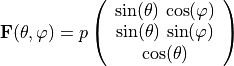
with ![\theta \in [0, \pi]](../../_images/math/d8fe4fa46b55d9ad117554e6bbafe71d7cd45f12.png) and
and ![\varphi \in [0, 2 \pi]](../../_images/math/60ff373055372c64ba28acaadb86a826aaee51c5.png) . The components of the total force vector
. The components of the total force vector  are
are
(41)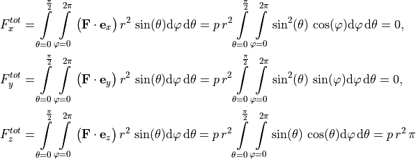
with  since we only integrate over one half of the shell.
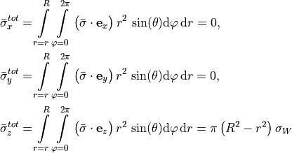
For the derivation of Laplace’s law we approximate the wall stress  by its mean value
  ,
see figure Fig. 134. Since the geometry and the acting forces are symmetric, the tangential stress in any
direction must be the same and there will be zero shear stress. Due to the assumption, the mean wall stress at the cut face
just acts just in z-direction, thus we have
,
see figure Fig. 134. Since the geometry and the acting forces are symmetric, the tangential stress in any
direction must be the same and there will be zero shear stress. Due to the assumption, the mean wall stress at the cut face
just acts just in z-direction, thus we have  and
and  .
The components of the total wall stress vector
.
The components of the total wall stress vector  are
are
(42)
with  . From equations (41) and (42)
we have
. From equations (41) and (42)
we have
(43)
From (43) we conclude that
(44)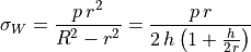
and for  we obtain the law of Laplace
(45)
which can be used to estimate the wall stress for thin walled spherical shells.
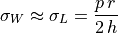
Modeling Error
The law of Laplace, see equation (45), is just an approximation to the more accurate formula
(44). The approximation is justified if the wall thickness is mush smaller than the inner
radius. To figure out how strong the relative modeling error depends on and , we rewrite the
error as
(46)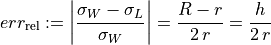
which yields to the condition

if we want to ensure that the relative modeling error is less than  .
.
Example
Assume, that we have a spherical shell with  and we want to use the law of Laplace,
equation (45), to estimate the surface tension. To ensure that the error is
less than one present, that is
and we want to use the law of Laplace,
equation (45), to estimate the surface tension. To ensure that the error is
less than one present, that is  , we have to ensure that the wall thickness
satisfies
, we have to ensure that the wall thickness
satisfies  . For
. For  we have
  and
for
and
for  we have
  .
.
Verification
To verify the stress, we first compute the stress tensor  elementwise and project the tensor from the
cartesian coordinate system to the spherical coordinate system, i.e.
elementwise and project the tensor from the
cartesian coordinate system to the spherical coordinate system, i.e.
(47)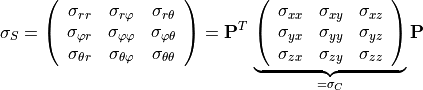
with the projection matrix 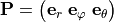 .
The mean stress tensor then is
.
The mean stress tensor then is
where the integration is applied componentwise.
Experiments
For the experiments we choose the following setups with two different geometries. The first geometry
is a thin walled spherical shell and the second geometry is a rather thick walled spherical shell.
The material model is the Demiray model with  ,
,  and
and  .
.
 [mm] [mm] |
 [mm] [mm] |
 [mm] [mm] |
 [kPa] [kPa] |
 [ms] [ms] |
|
|---|---|---|---|---|---|
| Experiment 1 | 15.0 | 15.5 | 0.5 | 2.0 | 100.0 |
| Experiment 2 | 15.0 | 15.5 | 0.5 | 4.0 | 100.0 |
| Experiment 3 | 15.0 | 30.0 | 15.0 | 2.0 | 100.0 |
| Experiment 4 | 15.0 | 30.0 | 15.0 | 4.0 | 100.0 |
Using the method described in this section, we obtain the following results.
 [kPa]
[kPa] |
 [kPa]
[kPa] |
 [kPa]
[kPa] |
 [kPa]
[kPa] |
 [kPa]
[kPa] |
|
|---|---|---|---|---|---|
| Experiment 1 | 39.2682 | 38.7745 | -0.9303 | 38.8500 | 38.8516 |
| Experiment 2 | 83.8585 | 84.8469 | -1.8753 | 83.7231 | 83.7220 |
| Experiment 3 | 0.6937 | 1.0304 | -0.3601 | 0.6260 | 0.6271 |
| Experiment 4 | 1.4428 | 2.1226 | -0.7198 | 1.2951 | 1.2973 |
We see, that for the thin walled geometry the analytically computed wall stress and
the Laplace approximation are almost equal to the computed mean tangential stresses
and . The radial stress is compared to the tangential stresses
negligible. The relative modeling error for the first two experiments are  and
and  , see equation (46).
For the experiments with a thick walled geometry we have a rather high discrepancy in the analytical
and computed stresses. The relative modeling errors for the last two experiments are
, see equation (46).
For the experiments with a thick walled geometry we have a rather high discrepancy in the analytical
and computed stresses. The relative modeling errors for the last two experiments are  and
and  .
.
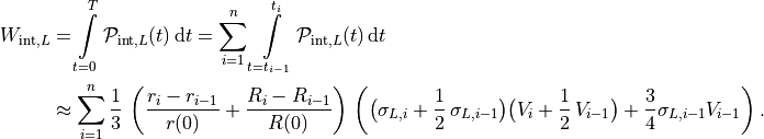
Work Verification
To verify the computed work, we compute the external work analytically and compare it with the computed
internal work. To compute the external work, we use the well known principle of
pressure-volume work
which is  where
where  denotes the volume of the inner sphere
(
denotes the volume of the inner sphere
(  ).
The integral representation then reads
).
The integral representation then reads
(48)
Next, we assume that the pressure is a piecewise linear function of the radius, that is
(49)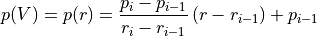
for ![r \in [r_{i-1}, r_{i}]](../../_images/math/939f8ccc871caa6cd37c4a853b9b7dfccf07592b.png) and
and  . We get the pressure and radius values
  from the
simulation.
from the
simulation.
Using spherical coordinates and equation (49), we can write equation (48) as
(50)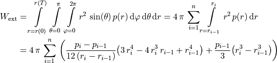
which provides an analytical approximation of the external work in [kPa mm^3] = 10^(-6) [J].
To compute the internal work, we use the internal mechanical power  which is
(51)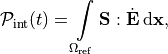
see [1] (Section 4.4) for further details. The internal mechanical work  is then given by
(52)
Note
The formula in [3] for the internal heart power and its modification yield
(53)
where  denotes the volume of the geometry at time
  and
and  denotes
the mean strain rate with the mean strain
denotes
the mean strain rate with the mean strain
 .
First, we assume that the stress, the volume and the radii depend piecewise linearly on time.
.
First, we assume that the stress, the volume and the radii depend piecewise linearly on time.
For the mean strain we obtain
(54)
with  and
and  . Thus, for , we have

with  and
and  .
.
By integrating over  we get

and finally for the internal work  we have
To obtain  we proceed in the same way by replacing with .
Experiments
Using the same geometrical settings as in Experiments we obtain the following results.
 [J]
[J] |
[J] |
[J] |
[J] |
|
|---|---|---|---|---|
| Experiment 1 | 0.00407 | 0.00420 | 0.00434 | 0.00428 |
| Experiment 2 | 0.01072 | 0.01112 | 0.01181 | 0.01167 |
| Experiment 3 | 0.00074 | 0.00070 | 0.00097 | 0.00065 |
| Experiment 4 | 0.00303 | 0.00285 | 0.00396 | 0.00268 |
Meshes
Download the following Python-script and run it!
References
| [1] | Holzapfel, G.A., Nonlinear Solid Mechanics: A Continuum Approach for Engineering (2000), West Sussex, England: John Wiley & Sons, Ltd |
| [2] | Grossman, W. and Jones, D. and McLaurin, L.P., Wall stress and patterns of hypertrophy in the human left ventricle (1975), American Society for Clinical Investigation |
| [3] | Fernandes, J.F. and Goubergrits, L. and Brüning, J. and Hellmeier, F. and Nordmeyer, S. and da Silva, T.F. and Schubert, St. and Berger, F. and Kuehne, T. and Kelm, M. and others, Beyond Pressure Gradients: The Effects of Intervention on Heart Power in Aortic Coarctation (2017), Public Library of Science |