Afterload Fitting
Module: tutorials.04_EM_tissue.06_afterload_fitting.run
Section author: Matthias Gsell <matthias.gsell@medunigraz.at>
Introduction
To provide suitable pressure boundary conditions for the EM-simulations, we use the three element Windkessel model to obtain the pressure trace from the volume. The three element Windkessel model is a simple model of afterload on the ventricle and can be written as the following ODE
(55)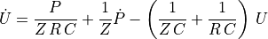
with  , where
  is the cavity volume and
 is the pressure in the ventricle. The constants
  are the parameters of the model, where
  is the Windkessel
series resistence,
is the Windkessel
series resistence,  is the parallel resistence and
  is the Windkessel capacitance.
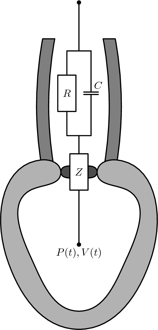
Fig. 140 Schematic depiction of the Windkessel model.
With a perfect dataset we can simpy derive  and by
plugging the pressure into eqution (55) and optimizing
and by
plugging the pressure into eqution (55) and optimizing
 and so that the simulated volume matches the clinical one.
In practice, it is more complicated, since the pressure traces and volume
traces are usually recorded on different days under different conditions.
Thus, to fit the Windkessel parameters,
and so that the simulated volume matches the clinical one.
In practice, it is more complicated, since the pressure traces and volume
traces are usually recorded on different days under different conditions.
Thus, to fit the Windkessel parameters,
- the Windkessel series resistence ,
- the Windkessel parallel resistence ,
- the Windkessel capacitance ,
we have to synchronise the pressure and volume data. For the synchronisation we can vary three synchronisation parameters,
- the time-offset between pressure and volume traces (
 ),
), - the pressure at which the aortic valve opens (
 ),
), - the scale factor applied to the volume trase (
 ).
).
In total we have to fit six parameters. As input parameters we have to provide
- a pressure beat,
- a volume trace,
- value ranges to perform the parameter sweep on (for the first five of the six parameters above),
- the end diastolic volume to be used.
Method
Using the data ranges provided by the user for the first five parameters listed above, a Latin Hypercube Sampling is used to construct a large parameter sweep. The sixth parameter is treated separately.
For each experimental design, the volume scale factor and the
time-offset are applied and used to construct a pressure-volume loop
(PV loop). From the aortic valve opening pressure in conjunction with the pressure trace,
we can determine the time at which the Windkessel solve should begin ().
Using the pressure trace, the Windkessel model (55) is solved with
parameters  and . The simulated volume trace is used to construct
a simulated PV loop which is compared to the clinical PV loop. This yields a cost for
each parameter set. The parameter set with the lowest cost is used to determine the fitted
Windkessel parameters and and synchronisation parameters.
and . The simulated volume trace is used to construct
a simulated PV loop which is compared to the clinical PV loop. This yields a cost for
each parameter set. The parameter set with the lowest cost is used to determine the fitted
Windkessel parameters and and synchronisation parameters.
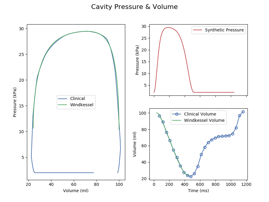
Fig. 141 Example of fit with lowest cost.
Usage
(Requires the pvprocess package)
For the windkessel tool in the pvprocess package several modes are available.
single: Solve a single Windkessel model using either synthetic pressure data or an input file.cavcheck: Validate the Windkessel model solution in a CARP cavity file.plotfit: Plot a previously fitted Windkessel model.fit: Fit a Windkessel model and its initial conditions.
To see the full option list of each mode run
windkessel <mode> --help
with the mode of your choice from the list above.
Fit
To run a Windkessel parameter fit as described above, we have to provide a pressure trace. This can be a measured pressure beat from a file
windkessel fit \                # the mode we want to run
--pressure-file pressure.json \ # the pressure file
--pressure-beat 5 \             # the pressure beat we want to use
--pressure-synthetic            # use this option if you want a smoothed pressure beat instead of the original one
or a synthetic pressure beat
windkessel fit \                # the mode we want to run
--pressure-synthetic \          # use synthetic pressure
--peak-pressure 22 \            # the peak pressure
--diastolic-pressure 2.5 \      # the pressure in the diastolic phase
--systolic-duration             # duration of the systole
when only the peak pressure is known. To provide the volume data, use
windkessel fit \                # the mode we want to run
--volume-file volume.json       # the volume file
or, alternatively you can use the -vf argument. In addition,
an ejection fraction and a duration may be provided to construct the cost
function using the options
windkessel fit \                # the mode we want to run
--fraction 51 \                 # the ejection fraction
--duration 300                  # the ejection duration
The arguments
-Z, -R, -C, --av-open-pressure, --av-open-pressure-absolute and
--time-offset take either one or two arguments, specifying either
a single value or a parameter range to sweep over. (--av-open-pressure
specifies the fraction of the peak pressure and --av-open-pressure,
where --av-open-pressure-absolute specifies the absolute value.)
The final input parameter is --ivc-volume to the initial value for
the Windkessel solve and should be the end diastolic volume of your model.
To enable parallel execution just set the number of processors with the
--np option. To specify the number of samples use the --samples
option. Finally, use the --info-json option to write the fitted
values to your file system.
Full Example
The following command performs a full Windkessel fit.
windkessel fit \
--pressure-synthetic \
--peak-pressure 29.46 \
--volume-file /PATH/TO/volume.json \
--systolic-duration 520 \
--av-open-pressure-absolut 10 11 \
-R 60 63 \
-C 38 40 \
-Z 75 79 \
--samples 10000 \
--np 10 \
--info-json tutorial.json