CvSys
Module: tutorials.04_EM_tissue.10_cvsys.run
Section author: Christoph Augustin <christoph.augustin@medunigraz.at>
Introduction
This tutorial guides through using the 0D Cardiovascular system simulator. The code is based on the CircAdapt model, see [Arts2005], [Lumens2009], [Arts2012], and [Walmsley2015].
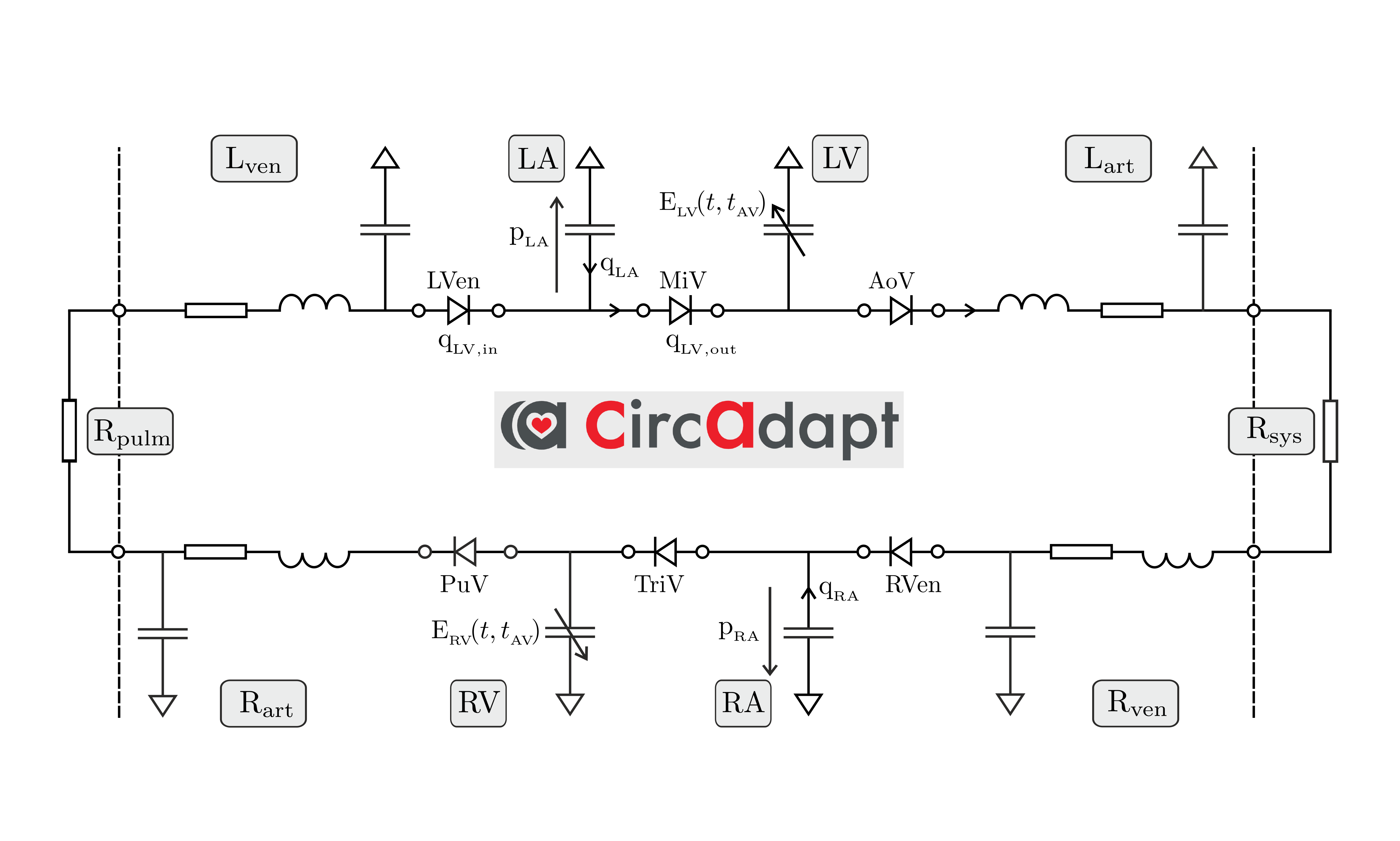
Fig. 155 Schematic of the 0D Closed-loop model CircAdapt
Usage
(Requires the cvsys package)
Basic Options
To see the full option list run
cvstool --help
The following basic options are available:
-h, --help              Display this information
-s, --solver <solver>   Choose ODE solver
                        Choices:
                          forw-euler: forward Euler method
                          rfk45: Runge-Kutta-Fehlberg 45
                          cvode: Sundials CVode solver
-d, --duration <float>  Duration of the simulation in (s)
                          default: 0.85 s
-o, --output <dir>      Place the output into the directory <dir>
--create-opts <file>    Create options file with default values
                          format choices are `json` and `prm`
                          default: `cvs_options.json`
--opts <file>           Use input options in <file>
The following command computes the heartbeat of a healthy adult over 60 seconds:
cvstool -d 60 \
        -o healthy_adult
Parameters of the cardiovascular systems can be changed using specific option files. First, generate options with
cvstool --create-opts cvs_options.json
Second, modify the options file cvs_options.json, e.g.,
set Aortic valve stenosis [pct.] to 70.
And third, simulate the heartbeat with a 70% aortic stenosis using the options file with
cvstool -d 60 \
        -o aortic_stenosis \
        --opts cvs_options.json
Post-processing
The cvsys experiment output information file on the cardiovascular system in
the chosen output folder in csv format. Depending on the cardiovascular
component these contain pressure information, volume information,
flow rates and many other additional informations.
These files can be used for a post-processing analysis using the tool cavplot.
Call
cavplot --help
for a detailed description of the usage.
The default output containts pressure-volume loops as well as pressure and volume traces
cavplot ./healthy_adult/cav.LV.csv
To plot a time interval of the output use --time-interval or --time
For example to plot the last two seconds of the simulation call
cavplot ./healthy_adult/cav.LV.csv --time-interval 58 60
To change the unit to mmHg use the flag --mmHg. To show PV loop and
pressure traces for the aortic stenosis case call
cavplot ./aortic_stenosis/cav.LV.csv --time 58 --mmHg
This should give you a plot similar to
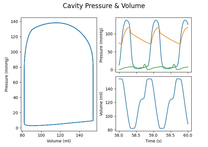
Fig. 156 cavplot output for the 70% stenosis case.
The options l+= and l= allow to add labels to the output.
To compare the pvloops for the healthy case and the case with 70% aortic stenosis
call
cavplot healthy_adult/cav.LV.csv:l="Healthy" \
        aortic_stenosis/cav.LV.csv:l="Aortic Stenosis" \
        --time 55 --mode pvloop
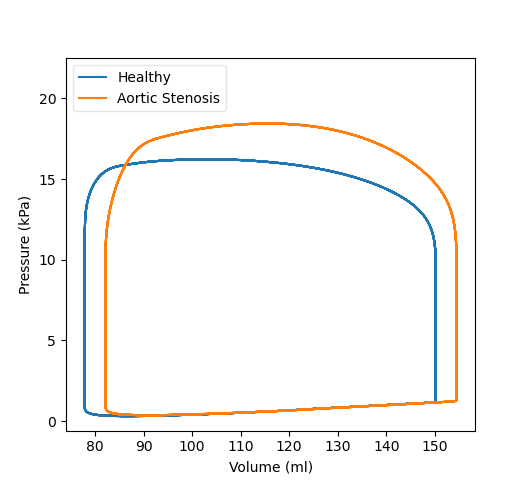
Fig. 157 Pressure-volume plot comparing the healthy and the stenotic case.
The option ls= in {dotted, dashdot, dashed, solid} allows to change the
linestyle. E.g., plot the pressure drop over the aortic valve:
cavplot aortic_stenosis/cav.LV.csv \
        aortic_stenosis/tube.AO.csv:ls=dashed \
        --time 55 --mode pressure
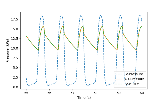
Fig. 158 Pressure-drop over the aortic valve.
The options v*=, p*=, and f*= allows to scale the volume(v), pressure(p),
and flux(f), respectively. The same also works for \=, and +=, -= for a
translation.
E.g. plot the flux over the pulmonary outlet, the mitral valve, volume change of
the left atrium in one plot:
cavplot aortic_stenosis/valve.PO.csv:f*=-1 \
        aortic_stenosis/valve.MV.csv \
        aortic_stenosis/cav.LA.csv:ls=dashed:l="LA Volume Change" \
        --mode flux --time 56.7 58.7
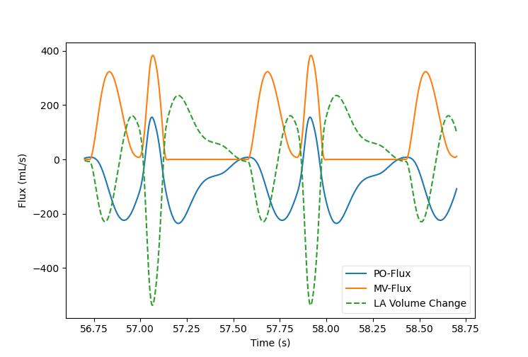
Fig. 159 Flux over pulmonary outlet and mitral valve and volume change of the left atrium.
Advanced Options
The following more advanced options are available:
--version <version>  Specify CircAdapt version to use (`2012`, `2015`)
                       default: `2015`
--no-peri            Run simulation without pericardium
--stiff-av-valves    Run simulation without updating leak area
                     of atrio-ventricular valves
--mass-conservation  Enable mass conservation
--allow-negative-p   Allow negative pressures in cavities
The different versions (2012, 2015) correspond to the publications [Arts2012] and [Walmsley2015], see also http://www.circadapt.org/downloads/files.
For example we can allow negative pressures in the cavities using
cvstool -d 60 -o healthy_adult_np --allow-negative-p
We plot the difference in the left atrial PV loop using the plotting option
c= that allows to change the color using RGB-HEX format
cavplot healthy_adult/cav.LA.csv:l="standard":c=#000 \
        healthy_adult_np/cav.LA.csv:l="allow-negative-p":c=#ff0000 \
        --mode pvloop --time 55 --mmHg
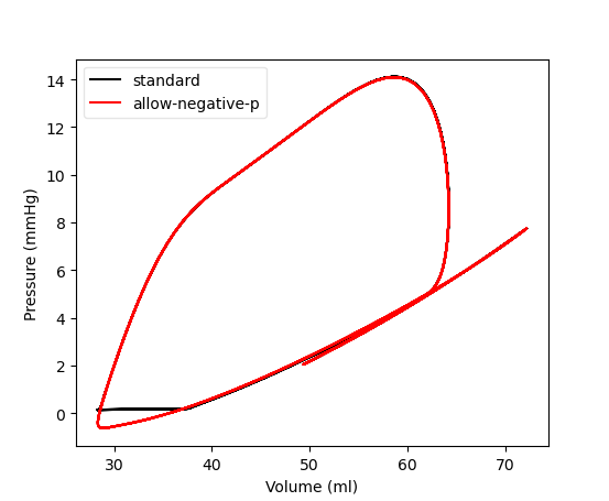
Fig. 160 Left atrial pressure with the standard code in black and with the
--allow-negative-p flag in red.
References
| [Arts2005] | T. Arts et al. AJP Heart 288 (2005): H1943-H1954. DOI: 10.1152/ajpheart.00444.2004. |
| [Arts2012] | (1, 2) T. Arts et al. PLoS Comput Biol 8 (2012): e1002369, DOI: 10.1371/journal.pcbi.1002369. |
| [Lumens2009] | J. Lumens et al. Ann Biomed Eng 37 (2009): 2234-2255, DOI: 10.1007/s10439-009-9774-2. |
| [Walmsley2015] | (1, 2) J. Walmsley et al., PLoS Comput Biol 11 (2015): e1004284, DOI: 10.1371/journal.pcbi.1004284. |