`Laplace-Dirichlet Rule-Based fiber and sheet generation.`

Module: tutorials.05_pre_post_processing.03_Laplace_Dirichlet_Fibers.run

Section author: Jason Bayer <jason.bayer@ihu-liryc.fr>

This tutorial demonstrates how to generate cardiac fiber and sheet orientation in biventricular models using the rule-based approach by [1].

Introduction

We developed a robust Laplace-Dirichlet Rule-Based algorithm for incorporating myocardial fiber orientation into computer models of biventricular geometries with speed, precision, and high usability. This tutorial demonstrates how to use the implementation of Bayer et al with CARP and its utilities.

Problem setup

Ventricular fiber and sheet orientation rules

In mammalian ventricles, the following rules for cardiac fiber orientation apply as derived from histological and diffusion-tensor imaging.

R1. The longitudinal fiber direction in the ventricular walls is parallel to the endocardial and epicardial surfaces.

R2. The longitudinal fiber direction rotates clockwise throughout the ventricular walls from the endocardium (+ $\alpha$ ) to the epicardium (- $\alpha$ ), where $\alpha$ is the helical angle with respect to the counterclockwise circumferential direction in the heart when looking from the base towards the apex.

R3. The longitudinal fiber direction in papillary muscles and trabeculae is parallel to the long axis of these structures.

R4. The transverse fiber direction is perpendicular to the longitudinal fiber direction and is defined by the angle $\beta$ , where $\beta$ is the angle with respect to the outward transmural axis of the heart.

R5. The sheet normal is orthonormal to the longitudinal and transverse fiber directions.

R6. Fiber orientation in the septum is continuous with the ventricular walls.

Laplace-Dirichlet method

To define the rules above in any finite element mesh of mammalian ventricles, we solve the solution to Laplace’s equation with Dirichlet boundary conditions for the four scenarios shown in the lefthand side of the figure below. We then use these solutions to develop the local coordinate system shown in the righthand side of the figure below. Tutorials for how to solve Laplace’s equation and gradients of scalar fields can be found at (TBA) and (TBA), respectively.

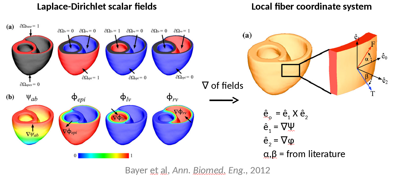
Using the local coordinate system derived by taking the gradients of the Laplace solutions, we then generate a longitudinal fiber direction according to user inputs for $\alpha$ on the cardiac surfaces, and the transverse and normal directions for sheet orientation according to the user inputs for $\beta$ on the cardiac surfaces.

Canine biventricular model

For this example, we use a finite element mesh of an adult canine biventricular geometry. The model is composed of 149,734 tetrahedral elements with an average edge length of 1.75 mm. This particular mesh was chosen since it’s lower resolution facilitates quick computation and visualization times. Note, all boundary conditions as shown in the figure above were computed beforehand using a customized tool. A tutorial for written in the near future.

Usage

The following optional arguments are available (default values are indicated):

./run.py --help 
  --mode              Options: {all,fibersonly}, Default: all
                      The option "all" computes the Laplace solutions
                      as well as the rule-based fiber orientation.
  --apex              Options: {apex_lv,apex_rvlv}, Default: apex_lv
                      The option sets the apical boundary condition either
                      at the LV apex or at the junction of the RV and LV.
  --alpha_endo        Default: 40  degrees
                      Helical angle on endocardial surface
  --alpha_epi         Default: -50  degrees
                      Helical angle on epicardial surface
  --beta_endo         Default: -65  degrees
                      Sheet angle on endocardial surface
  --beta_epi          Default: 25  degrees
                      Sheet angle on epicardial surface

After running run.py, the results for the fiber orientations can be found in the output subdirectory corresponding to the input parameters. The longitudinal fiber direction can be found in canine_long.vec, the transverse direction in canine_tran.vec, and the sheet normal direction in canine_norm.vec.

If the program is ran with the --visualize option, meshalyzer will automatically load the longitudinal fiber orientation.

Tasks

Generate fiber and sheet orientation using the apex_lv boundary condition.

./run.py --apex apex_lv

Generate fiber and sheet orientation using the apex_rvlv boundary condition.

./run.py --apex apex_rvlv

Visualize a purely circumferential longitudinal fiber orientation.

./run.py --alpha_endo 0 --alpha_epi 0

Visualize a purely apicobasal longitudinal fiber orientation.

./run.py --alpha_endo 90 --alpha_epi 90

Literature

[1]	Bayer JD, Blake R, Plank G, Trayanova NA. A Novel Rule-Based Algorithm for Assigning Myocardial Fiber Orientation to Computational Heart Models. Annals of Biomedical Engineering, 40(10):2243-2254, 2012. [Pubmed]