IGB tools
Module: tutorials.05_pre_post_processing.05_igbutils.run
Section author: Edward Vigmond <edward.vigmond@ihu-liryc.fr>
This tutorial demonstrates several utilities to manipulate IGB files.
Introduction
The IGB format is used by CARPentry. For a complete description of this format see the meshalyzer manual. We have developed many tools to handle the IGB format files, and these tools have been designed to run in parallel where possible, as well as be aware of memory limits when processing large files. Options are listed with the -h or –help option. Some commands give more details with –detailed-help.
Parallel Usage
OpenMP is used for parallelizing some computations. Thus, to run the utilities in parallel, make sure that you set the following environment variable:
export OMP_NUM_TREADS=12
where, instead of 12, you can set it to however many processors that you would like to use.
The utilities
| Progam | Purpose |
|---|---|
| igbhead | display and edit the header, convert data type |
| igbextract | extract data from a subset of nodes in an IGB file with various output formats |
| igbops | perform mathematical operations on an IGB file |
| igbapd | compute action potential durations |
| igbdft | perform frequency domain operations |
| GlGradient | take the gradient of a data field, and compute velocity |
igbhead
Simply supplying the IGB file displays all the metadata
linux-iokj%igbhead vm-2.5-1.5-600.0.igb
x dimension:    201
y dimension:    1
z dimension:    1
t dimension:    25001
data type:      float
Pixel units:    mv
Pixel zero:     0
Pixel scaling:  1
X units:        um
Y units:        um
Z units:        um
T size:         25000
T units:        ms
Increment in t: 1
T origin:       0
Created on:     little_endian
The fields x, y and z are the number of pixels in each direction for structured meshes. For unstructured meshes, it is only their product which matters.
Note
Do not set any of them to zero or meshalyzer will complain
Setting any field changes its value in the header but does not touch the data. To actually convert data from one type to another, from float to half-float for example, the flag specifying to change the data must be added:
igbhead --convert-data --data-type=hfloat -f half_float.igb float.igb
ASCII files may be converted to IGB format. The ACSCII file must have one line per time instance and each line contains white space separated values. The user is expected to know the number of nodes (N) and the number of time instances (T):
igbhead -xN -y1 -z1 -tT -dfloat --create -fa.igb data.txt
igbextract
This is a fairly useful utility that can extract a subset of the time series from any distributions of nodes. It can output in several formats, some ASCII, binary or another IGB file. For example:
igbextract -n 0,100-110,500 --t0=100 ---t1=2000 a.igb
will output times series from the period 100 to 2000 ms from the nodes 0, 100-110 inclusive, and 500 as an ASCII file wherein each line begins with the time and each subsequent field is the value at the node at that time.
| Format | Explanation |
|---|---|
| IGB | IGB file |
| binary | raw data, 4 byte floats |
| asciiTm | on each line, time followed by nodal values |
| ascii | on each line, nodal values at one time |
| dat_t | auxilliary data format. See meshalyzer manual |
| ascii_1pL | one nodal value per line |
igbops
This is a general utility to perform mathematical operations, including those between two IGB files.
It supports a number of built-in operations, controlled by parameters a and b.
Arbitrary expressions can also be specified with the
expr option which uses
mu parser for compiling the expression.
Given that X has the dimensions in space and time of [n,t], Y can have dimensions below
| Y | Application |
|---|---|
| [n,t] | Y applied point by point over space and time to X |
| [n,1] | The same Y is applied point by point to each time frame of X |
| [1,t] | Y changes at each time instance but the one same Y value is applied to all X points |
igbops commands can be piped together to perform several calculations without storing intermediate files. In this case, input and/or output filenames are given as - to signify stdin and stdout. Y must be a file and cannot be read from stdio:
igbops --expr "sqrt(10*X+Y)" a.igb b.igb -O- | igbops --op maxX_i -
Here is an example to normalize some optical mapping data contained in vm_opt.igb:
# find the minimum value at each node -> minopt.igb
igbops --op=minX_i --output-file=minopt vm_opt.igb
# find the range at each node = max - min - > range.igb
igbops --op=maxX_i --output-file=- vm_opt.igb | igbops --expr='X-Y' -Orange - minopt.igb
# shift the minimum of each signal to zero and then divide by the range -> vm_norm.igb
igbops --op=aX+bY --a=1 --b=-1 -O- vm_opt.igb minopt.igb | igbops --op=XdivY -Ovm_norm - range.igb
igbapd
This utility computes action potential duration (APD). Several parameters can be specified to change if an AP is detected and how the APD is defined. There are three modes of operation:
| mode | output |
|---|---|
| all | output all APDs in order of detection, specifying the node at which an AP was detected |
| first | only detect first AP at each node, output APDs in node order |
| detect | indicate node at which first AP is detected |
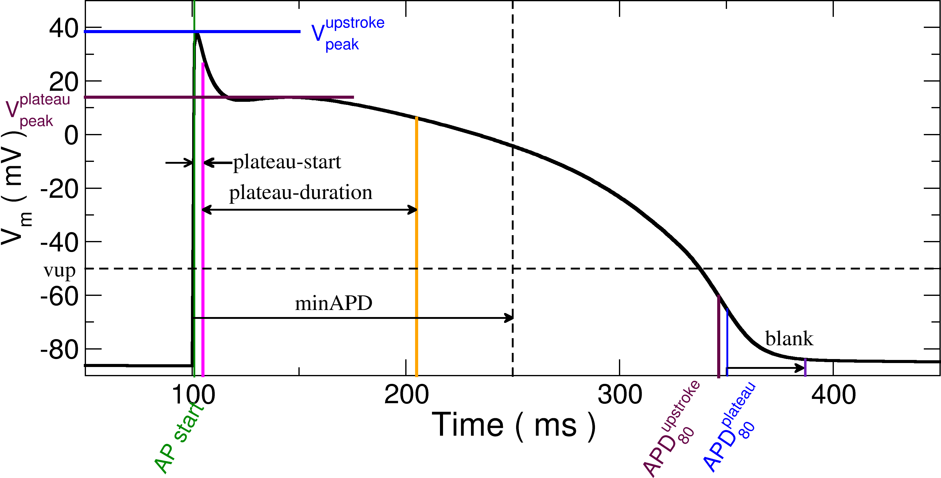
The start of an action potential is defined when a threshold voltage (vup) is crossed with the rate of change of voltage
also exceeding a prescribed threshold (dvdt).
To determine the peak value of the AP, either the initial spike may be used (upstroke) or the peak value of the plateau (plateau).
In the case of the maximum plateau value, the start of the plateau is defined as a delay after the upstroke
(--plateau-start) and its duration is defined by --plateau-duration.
The action potential must be longer than minapd or it is discarded.
A blanking period may be specified after the end of an AP to prevent spurious detections.
AP traces will not be analyzed for the period specified by --blank.
The diagram below shows the relevant parameters:
igbdft
This utility performs frequency domain operations.
| Operation | Meaning |
|---|---|
| DomF | calculate the dominant frequency of each node |
| Butter_bp | Butterworth bandpass filter. Specify 0 for a limit to ignore it. |
| phase | Perform Hilbert transform to calculate instantaneous phase. Heavy low pass filtering is recommended. |
| PSD | Power spectral density of each node |
| notch | perform notch filtering |
GlGradient
This is extremely useful for taking the gradient but also computing propagation velocities as well. The most accurate method is to compute the activation times by including the following options in your CARP simulation:
numLATs = 1
lats[0].all = 0
This will produce a file of activation times, linearly interpolated to less than the time step resolution.
By default, a file called init_acts_vm_act-thresh.dat will be produced. The propagation velocity  is computed from the activation time,
  by
by

To use GlGradient given results are on model.pts:
GlGradient --meshname=model --data=init_acts_vm_act-thresh.dat -c8 --velocity
Exercises
Exercise #1: igbapd
Computing APD is essential for EP studies. To practice computing APD with igbapd for CARP simulations, a simulation in a 2D cable is provided in the directory ./Cable_Mesh_APD, along with a vm.igb file containing 10 seconds of simulation during 1Hz pacing at one end of the cable. Load the simulation in meshalyzer and visualize the action potentials at each node using the time series button under the highlights tab. If you do not see the cable, turn on connections.
Using these files, compute both the first and last APD for the cable. What do you notice about APD in the middle of the cable between these beats? Is it longer or shorter?
Secondly, computer APD for all other beats. How does APD change for sequential beats? Does it eventually stabilize?
Lastly, recompute APD using the -v option upstroke instead of plateau. What happens to APD near the stimulus region when computing APD with the upstroke? Why is this so?
To see the answers, please run the following commands
Compute APD for the first beat.
run.py --answer igbapd --mode single --beat 1 --peak plateau

Compute APD for the last beat.
run.py --answer igbapd --mode single --beat 10 --peak plateau

Computer APD for the first beat, but with upstroke option.
run.py --answer igbapd --mode single --beat 1 --peak upstroke

Compute APD for all beats. Note, the output will appear in the terminal.
run.py --answer igbapd --mode all --peak plateau
To practice further, you will need to go to the directory for the Periodic Boundary condition tutorial 02/07B and run the following command:
run.py --size=2 --tend=400 --bc=Yper --monitor 10 --np=4 --block-dur=99
Now, measure the first APDs and plot them in meshalyzer. Compute all APDs and look at the file format
Exercise #2: igbextract and igbops
We wish to compute bipolar electrograms from a set of unipole electrograms that we have created using phie recovery. Provided for you in the tutorial directory are the unipolar points file (unipolar.pts) and the corresponding EGMs recorded at these points (unipolarEGMs.igb). Note, the electrogram pairs are adjacent in the file. Using these files, how can we generate an IGB file of bipolar electrograms using igbops and igbextract? Hint, as the option suggests, you will need to both igbextract and igbops.
To obtain the answer, run the following
run.py --answer igbextract+ops
Note, if you want to see the vertices in meshalyzer you will need to increase their size, and you can use the time series button to visualize the potential traces on each node.
Exercise #3: GlGradient
Computing gradients in a nonuniform mesh is a very useful tool. To become familiar with this function, complete the following.
-Generate a the carp files .pts, .elem, and .lon for a single element of your choice
-Generate a .dat file with scalar data on each node
-Run GlGradient on this mesh to compute the gradient at the center of the element.
-Visualize the gradient in meshalyzer using the load vector option. Note, you will need to generate a .vpts file with the element center point to accompany the output .vec file containing the gradient vector. The file formats are discussed in the meshalyzer manual.
What happens to the gradient vector when you change the values of scalar data? What direction does it point? Furthermore, how does the magnitude of the gradient change? You can find the option for output the magnitude under the –help options. Note, the latter is very important for such tasks as computing local conduction velocity. Run -help to see all options.
To see how this is done for a single quadrilateral element with scalar values of 1 at the top of the element, and 0 at the bottom, run the following command
run.py --answer GlGradient --QNd_0 0 --QNd_1 0 --QNd_2 1 --QNd_3 1
You can adjust the arrow size of the vector under the Vectors tab.
Exercise #4: igbdft
Computing dominant frequency is a useful tool in EP simulations, particularly to study reentry. For example, dominant frequency maps can help locate the main reentrant circuits driving arrhythmia in cardiac tissue. To illustrate this point, a simulation of reentry (vm.igb) in a 2D cardiac slab (mesh.pts) is provided for you in the directory ./Slab_Mesh_VF. Please visualize this brief episode of reentry in meshalyzer and visually locate the reentrant sources and the frequency of rotation. After, use igbdft to compute the dominant frequency and see if the output corresponds to what you found.
To see the solution, please run the following
run.py --answer igbdft