`UVC Applications`

Module: tutorials.05_pre_post_processing.07_UVC_applied.run

Section author: Edward Vigmond <edward.vigmond@ihu-liryc.fr>

Applying UVCs

This tutorial demonstrates how to apply UVCs.

Introduction

UVCs allow one to easily define structures on a mesh or transfwer data between two meshes. We can view UVC space as the reference frame and as such, transferring from Cartesian to UVC space is a pull operation, and going the other way is a push.

If transferring scalar data between meshes, it suffices to have the UVCs of where the data is on the source mesh, and interpolate based on UVC positions on the destination mesh.

For transferring gradients and directions, the quantities are vectors which are first pulled to UVC and pushed to Cartesian making use of the deformation gradient. In these cases, the deformation gradient is calculated by taking the gradient of the UVCs with respect to the Cartesian coordiantes. Care must be taken performing the calculation for the $\phi$ coordinate because of the branch cut at $\pi$ . Even though the value $\phi$ decreases when going clockwise, crossing from $\pi$ to $-\pi$ , the gradient is still positive because we need to ignore the branch cut and continue to increase $\phi$ above $\pi$ .

The program closest_hc_wf.py is capable of these mappings. To see how to use the program, detailed help is available:

closest_hc_wf.py -h

Applications

The generation of UVCs for a particular mesh should have been previously described. This tutorial will describe how to use UVCs to define location generically and how to transfer data.

Looking at the experiment specific options:

--line Z0 R0 PHI0 Z1 R1 PHI1 V
                      define a line by start and end points (default: None)
--n-line-pts N_LINE_PTS
                      number of points in each line [50]
--box-region Z0 R0 PHI0 Z1 R1 PHI1 V LABEL
                      define a region by bounding box and give a label to it
                      (default: None)
--expr-region EXPRESSION REGION_VALUE
                      include points (Z,R,P,V) satisfying specified python
                      expression (default: None)
--transfer UVCs DATA  UVC points on to which data is to be transferred
                      (default: None)
--mesh MESH           mesh on which to define objects [canine]
--UVC UVC             UVC file for mesh [dog_vtx]
--scale SCALE SCALE   scaling for UVC search (default: [3, 0.3333])
--IDWpower IDWPOWER   inverse distance weighting power (default: 2)
--numf NUMF           number of closest points to find (4)

Lines

Lines can be defined in UVCs by giving their starting and ending coordinates (except $\nu$ which is specified at the end). The option can be given multiple times to define multiple lines. The parameters are linearly interpolated between the specified end points. Set $\nu$ to -1 for the LV and 1 for the RV. Example: 0 0 -3.141 .5 0 0 -1 for an endocardial line in the lower half of the LV.

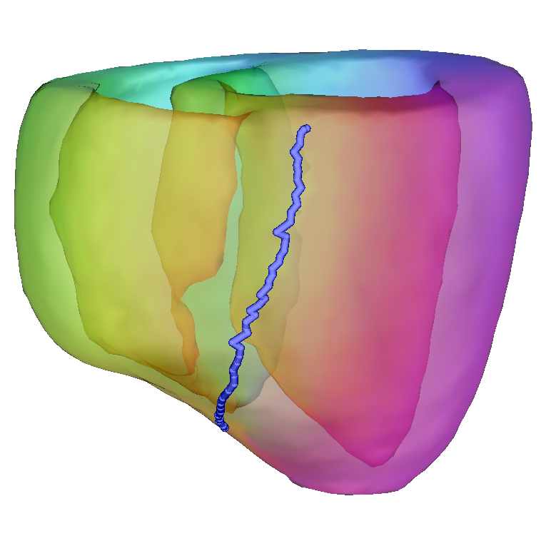
Fig. 165 A line defined by run.py –line 1 1 1.57 0.12 1 1.57 -1 –numf 25 –scale 2 .7 –IDW 1. $\phi$ data is displayed on the surfaces.

Bounding Box Regions

Like lines, the region option can be given multiple times to define multiple regions by bounding boxes in UVCs. Any point in the bounding box is tagged as within the region. Again, it is assumed that the region lies only in one ventricle so one $\nu$ value is specified after the other coordinates. A region label is also expected which is simply an identifying integer.

Expression Regions

Regions may be defined by expressions as well. Expressions are written as Python functions of Z, R, P, and V which refer to the UVC coordinates $\mathfrak{z}$ , $\rho$ , $\phi$ , and $\nu$ respectively. The function is evaluated at each coordinate and those coordinates evaluating to a true result are added to the region. A value for the region is also required. Examples:

The lower half of the RV: Z<0.5 and V>=0
The LV freewall endocardium: R<0.1 and V<=0 and (-3.1415926<P<-1.57 or 3.1415926>P>1.57)

Controlling Interpolation

Interpolating on to the new points from the known is performed using Shepard’s formula, that is, inverse distance weighting to an exponent. The exponent on the distance can be controlled with --IDWpower. The number of the nearest points to use for interpolation is controlled by --numf. The distance between points A and B in UVC space is determined by

$d(A,B) = \sqrt{ S_{\mathfrak{z}}(\mathfrak{z}_A-\mathfrak{z}_B)^2 + S_{\rho} (\rho_A-\rho_B)^2 + (\phi_A-\phi_B)^2}$

where $S_{\mathfrak{z}}$ and $S_{\rho}$ can be set with --scale. Usually 3 0.3 is reasonable.

Exercises

Note

The dog mesh is low resolution which accounts for some of the jaggedness of results.

Define the LAD as a line
Define the circumflex artery. You may have to use more than 1 line and cross ventricles.
Define a full thickness, RV free wall scar region covering the middle third in the apical basal direction.
Try using an expression to define a circular region of radius r centered at (B,*,A,1) with something like:
```
run.py --expr-region '((P-A)**2 + (Z-B)**2 < r**2) and V>=0' 2 --vis
```
Replace A, B and r with apropriate values. You may need to scale in a direction to get it more circular.
Transfer the dog mesh Z coordinates to the rabbit mesh. First extract the Z coordinates from the UVC file of the dog:
```
awk '{print $1;}' dog_vtx.pts | tail -n +2 > dog_z.dat
```
Define a region on the dog and transfer it (region.dat) to the rabbit

Literature

[1]	Bayer et al., Universal ventricular coordinates: A generic framework for describing position within the heart and transferring data, Med Image Anal, 45: 83-93, 2018. [PubMed] [Full]