Visualization Tools

Installation

Meshalyzer uses the Fast Light Tool Kit (“FLTK”) to provide modern GUI functionality. It supports 3D graphics via OpenGL ^TM and its build-in GLUT emulation. Before getting the software from a GitHub repository, a version 1.3.x of FLTK needs to be provided on your system by either installing it through the package manager or compiling it from the sources:

cd <installation-directory>
wget http://fltk.org/pub/fltk/1.3.4/fltk-1.3.4-1-source.tar.gz
tar -xzvf fltk-1.3.4-1-source.tar.gz
cd fltk-1.3.4-1
./configure --enable-xft --enable-shared
make
sudo make install
cd ..

Hence, get Meshalyzer from the freely available GitHub repository and finish your installation.

cd <installation-directory>
git clone https://github.com/cardiosolv/meshalyzer
cd meshalyzer
make

Input Files

Meshalyzer assumes that there is a model, defined by a set of vertices, which is to be displayed. Beyond that, everything is optional. The vertices may be connected to form structures, specifically cables, triangular elements, quadrilaterals, tetrahedra, hexahedra, prisms, or simple line segments. Scalar data may be associated with every point on the grid and may be used to colour any of the connected structures. An auxiliary set of points may also be defined on which to display vector data,

Furthermore, the points may be divided into different regions which may have their attributes independently manipulated. Regions are delimited by tagged volume elements (see Sref{sec:voleles}), or may be specified by a range of vertices (see~Sref{sec:regfile}), As well, all the structures formed by those vertices are part of the region. Vertices may belong to more than one region, and there is at least one region in a grid. If a region is not specified, all structures belong to the default region. If there is a element direction file (.lon file), and no volume elements are tagged, elements with no direction will be region 0, and other elements will be region 1.

Surfaces may be formed from collections of two-dimensional elements. Surfaces are defined by surface element files (see Sref{sec:surffile}). Also, surfaces are defined if there are any 2D elements in an elem file (see Sref{sec:elem}). In the latter case, the 2D elements are placed in different surfaces based on their region number. Surfaces are independent of regions, and the relationship between the points and model structures is described in the fig-UML.

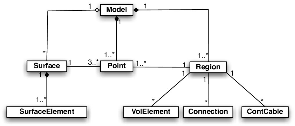
Fig. 12 Relationship between vertices (Points) and other structures.}

All files (except IGB files) are ASCII files. They may be gzipped in which case .gz should be appended to the extensions given below. Note that files are scanned line by line and that extra information on each line is ignored by meshalyzer.

Installation

Go to the ParaView homepage and choose your platform.

• Linux For Linux systems just download the archive file and extract its contents. Then run

  cd /PARAVIEW/PATH/bin
  ./paraview
  

• Windows For Windows systems download the installer and run it! After the installation finished, run Paraview by clicking on the Paraview icon.

• Max OS No idea at all!

Overview

After a successful installation and after you managed to run ParaView, you may load data sets to visualize. The standard file format is the VTK file format. A detailed user guide is available as pdf. In the following only a few of the most basic operations are illustrated.

1. Data Sets and Filters: List of all data sets and filters, toggle visibility by clicking on the eye icon next to the data set / filter.
2. Pipeline Browser: The pipline browser summarizes all the used data.
3. Common Filters: In this toolbar you can find the most commonly used filters in ParaView. They include (from left to right): Calculator, Isosurfaces, Clipping, Slicing, Thresholding, Subset Extraction, Glyphs, Streamlines, Wraping, Dataset Grouping, and Level Extraction.
4. Active Variable Controls:
5. Representation Toolbars:
6. Camera Controls:
7. VCR Controls and Current Time Controls:
8. Filters:
9. Properties:
10. Animation View:
11. Selection Tools:

Filters

To process data, a broad variety of filters is available. In the following we want to explain the most important of them.

Calculator

This filter is rather useful for postprocessing data. For example when you want to calculate the total pressure for some CFD data .

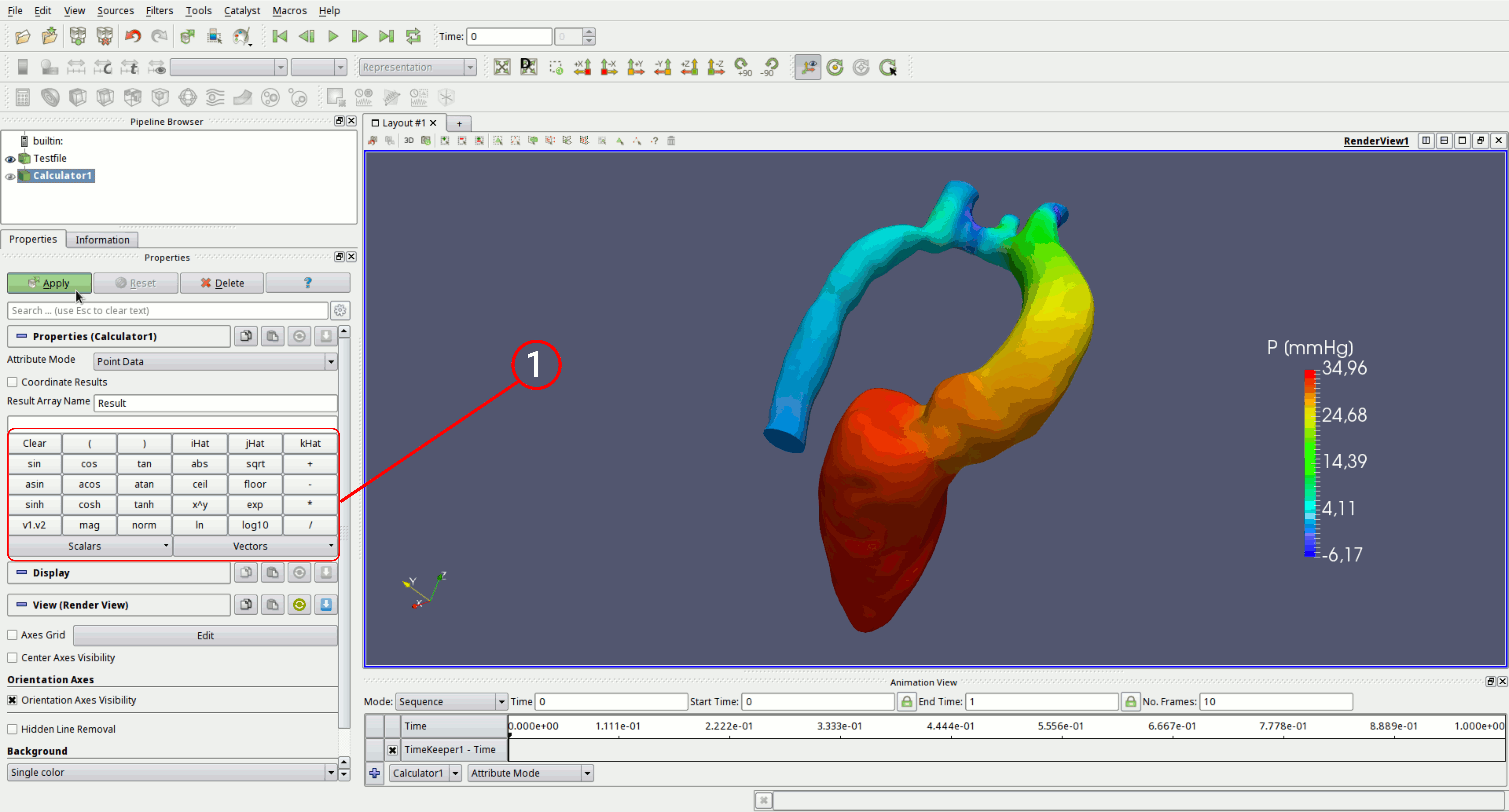
1. Here you find listed some build in mathematical expression. The buttons labled iHat, jHat, kHat denote x,y,z coordinate vectors (if you want to build together a vector valued function of your own.
2. You can switch here for a nodal based result or a cell based result
3. Here you chose from your loaded data. Can either be nodal based or cell based

For real Python-Afficiniados there is also a Python extension of this calculator to directly manipulate the data arrays.

• Cell Data To Point Data : Map cell data to point data on unstructured data sets.
• Clip : Clip the data set.
• Contour : Draw contour surfaces.
• Extract Selection : Extract selected points or elements.
• Glyph : Draw glyphs for a vector valued data set.
• Gradient Of Unstructured DataSet : Compute the gradient for a unstructured data set.
• Iso Volume : Draw the volume
• Point Data To Cell Data : Map point data to cell data on unstructured data sets.
• Slice : Slice the data set.
• Stream Tracer : Draw streams for a vector valued data set.
• Threshold :
• Warp By Scalar : Warp geometry by scalar data set.
• Warp By Vector : Warp geometry by vector valued data set.