`Smooth gradient heterogeneities (ionic adjustment)`

Module: tutorials.02_EP_tissue.05E_Smooth_Gradient_Heterogeneities.run

Section author: Patrick Boyle <pmjboyle@gmail.com>

This tutorial details how to assign a gradient of cell-scale properties using the adjustments interface.

Problem Setup

This example will run one simulation using a 2D sheet model (1 cm x 1 cm) in which all elements and nodes are in the same imp_region[] and gregion[] but heterogeneity in cell-scale dynamics is imposed at the cell scale in gradient patterns using the adjustments interface.

By default, $I_{Kr}$ is modulated from 0x to 5x from left to right and $I_{to}$ is modulated from 0x to 5x from bottom to top. Both gradients are linear. The resulting pattern of excitation is shown below:

../../_images/05E_Smooth_Gradient_Heterogeneities_Fig1_Animation.gif

Fig. 92 Membrane voltage over time ( $V_m(t)$ ) for the example in which $I_{Kr}$ is modulated from 0x to 5x from left to right and $I_{to}$ is modulated from 0x to 5x from bottom to top. Different-coloured stars indicate points where AP traces are shown in the graph below (Fig. 93).

The stars are colour-coded and indicate the approximate locations from which the action potential traces shown below were extracted:

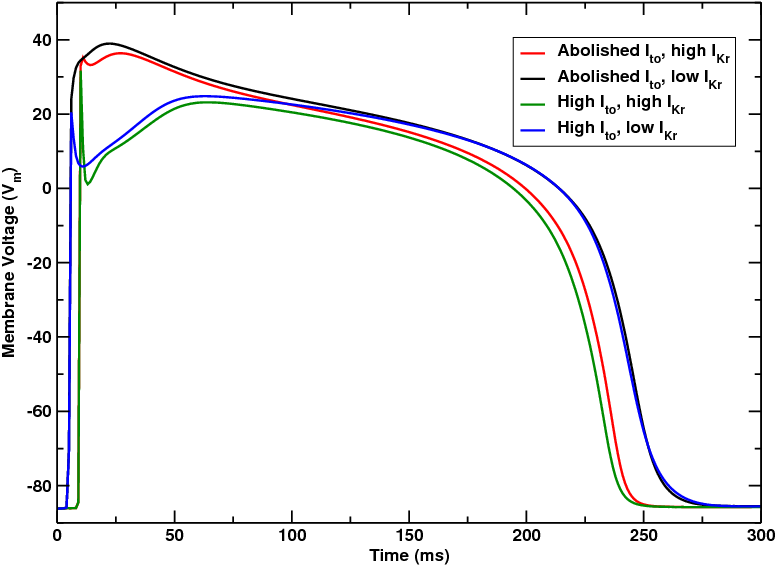
../../_images/05E_Smooth_Gradient_Heterogeneities_Fig2_Example_APs.png

Fig. 93 Action potential traces extracted from the four points indicated in Fig. 92.

As expected, $I_{to}$ modulation leads to an abolished notch along the bottom edge of the sheet but an exaggerated notch along the top edge. $I_{kr}$ modulation in the sheet leads to a progressive shortening of action potential duration from left to right as more repolarizing current becomes available to the cells.

Usage

The following optional arguments are available (default values are indicated):

./run.py --help 
  --xgrad_var         Options: {GCaL,Gks,Gkr,Gto}, Default: Gkr
                      parameter that should be varied along the left-to-right (X) gradient
  --xgrad_left_scf    Default: 0.0
                      scaling factor at left side of the X gradient
  --xgrad_right_scf   Default: 5.0
                      scaling factor at right side of the Y gradient
  --xgrad_flip        left becomes right, right becomes left

  --ygrad_var         Options: {GCaL,Gks,Gkr,Gto}, Default: Gto
                      parameter that should be varied along the bottom-to-top (Y) gradient
  --ygrad_bottom_scf  Default: 0.0
                      scaling factor at bottom of Y gradient
  --ygrad_top_scf     Default: 5.0
                      scaling factor at top of Y gradient
  --ygrad_flip        down becomes up, up becomes down

If the program is run with the --visualize option, meshalyzer will automatically load the $V_m(t)$ sequence corresponding to the run simulation. Output files for activation and repolarisation sequences as well as APD are produced for each simulation and can be found in the output directory and loaded into meshalyzer.

The –xgrad[…] and –ygrad[…] parameters can be modified to impose different gradients in the x and y directions (i.e., left-to-right and bottom-to-top, respectively) in four different parameters: $g_{CaL}$ , $g_{Ks}$ , $g_{Kr}$ , and $g_{to}$ , which correspond to the L-type $Ca^{2+}$ , slow delayed rectifier $K^{+}$ , rapid delayed rectifier $K^{+}$ , and transient outward $K^{+}$ currents, respectively.

Notes and Precautions

The --xgrad_var and --ygrad_var parameters should not be set to the same value, otherwise the simulation will not behave as expected.
The -adjustments[] interface in CARP can only be used to modify cell-scale properties that correspond to a state variable in the ionic model being used.

Use the –imp-info argument of bench to find out which variables are eligible to bet set on a nodal basis. There are actually two types of variables listed as state variables, (1) actual state variables which describe the ionic model state and evolve with each time step, and (2) model parameters which affect behaviour but do not change. Thus, state variables can be intialized on a nodal basis. Parameters which can be set on a nodal basis must be listed as parameters, i.e., being listed up top, as well as being listed as state variables. For example, in the case of the converted_TT2 ionic model used in this example, the following are parameters which can be set nodally:

> bench --imp=converted_TT2 --imp-info
converted_TT2:
[...]
      State variables:
                              GCaL
                               Gkr
                               Gks
                               Gto

Under the Hood

In the parameter file, the following options are used to adjust nodal values. First, if you wish to adjust N variables:

num_adjustments = N

For each adjustment structure, i.e., adjustment[0], ..., adjustment[N-1], the following fields are set:

Field	Meaning	Value
file	file specifying adjustment	see the Vertex adjustment file format
variable	variable to adjust	There are 2 forms. For global variables (Vm,Lambda,delLambda,Na_e,Ca_e,…) it is simply the variable. For ionic model state variables, it takes the form `X.Y` where `X` is the ionic model and `Y` is the state_variable, eg., `converted_TT2.Gto`
dump	output adjusted values on grid	0\|1