`Extracellular potentials and ECGs`

Module: tutorials.02_EP_tissue.07_extracellular.run

Section author: Gernot Plank <gernot.plank@medunigraz.at>, Fernando Campos <fernando.campos@kcl.ac.uk>

Overview

This tutorial explains the background of computing extracellular potentials and ECG using different techniques. The techniques used have their specific advantages depending on the application scenario. In this tutorial the focus is on using $\phi_{\rm e}$ to compute unipolar extracellular electrograms and compare these with fullblown bidomain simulations.

Recovery of extracellular potentials: Recovery techniques are efficient when potentials shall be computed for a limited number of field points. An important limitation is the underlying assumption that cardiac electric sources are immersed in an unbounded conductive medium of conductivity $\sigma_{b}$ . The technique is not overly efficient for a large number of field points such as in a body surface potential mapping application. There BEM-based or lead field approaches are better suitable.
bidomain: When using a bidomain formulation extracellular current flow and potentials are computed everywhere in the entire domain. This approach is most accurate and considered a gold standard for ECG modeling. However, the main disadvantage is the significantly increased computational cost. First, the entire domain must be explicitly discretized, that is, the tissue domain plus a bath or torso domain where extracellular potentials can be recorded. Secondly, bidomain requires the solution of an elliptic PDE which tends to be more costly than the plain reaction-diffusion monodomain equation, roughly by one order of magnitude.
pseudo bidomain: In this case very similar considerations hold as in the bidomain case. The main advantage of a pseudo-bidomain approach as published by Bishop & Plank are the significant savings in computational cost. A pseudo-bidomain is only marginally more expensive than a monodomain simulation as extracellular potentials are only solved at output granularity. The main disadvantage of the pseudo-bidomain approach is that any feedback of current flow in the extracellular medium upon excitation spread remains unaccounted for. This shortcoming can be alleviated though by using augmentation which takes into account the increased conductivity along tissue surfaces in presence of a bath of higher conductivity.

Theoretical background and more rigorous validation of the methods are found in the electrocardiogram section of the manual and in [1] and [2].

Objectives

This tutorial aims to achieve the following objectives:

Understand how to use the CARPentry $\phi_{\rm e}$ -recovery feature
Analyse differences between $\phi_{\rm e}$ -recovery and full bidomain-based extracellular potentials
Examine the effect of bath size upon extracellular potentials in the bath medium and its relationship to recovered potentials.

Setup

A simple reduced wedge setup is used for this tutorial. While a reasonable transmural width of 10 mm is used, in the circumferential direction the spatial extent is limited to the used spatial resolution for the sake of computational efficiency. That is, the wedge is a 3D object, but comprises only one layer of elements along the circumferential direction (x-axis), rendering the setup almost 2D. The wedge contains transmural as well as apico-basal heterogeneities which are based on the study of Boukens et al [3]. The wedge uses standard transmural fiber rotation. Stimulation sites to initiate propagation can be chosen at six different locations along the endocardial and epicardial surface. The size of the bath is exposed as an input parameter and can be varied. An overview of the experimental setup is given in fig-tutorial-ecg A). Default visualization outputs showing local activation time, action potential propagation and extracellular potentials are illustrated in fig-tutorial-ecg B).

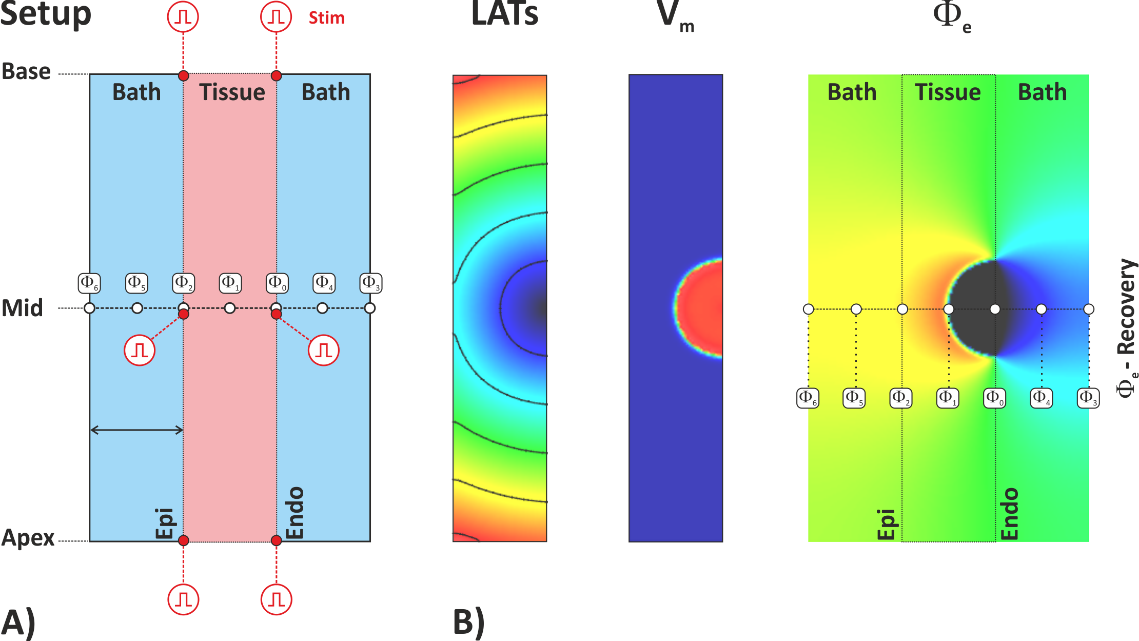
../../_images/Tutorial_EP_tissue_07_ecg.png

Fig. 95 Computing extracellular potentials and ECGs. A) Setup B) Visualization Extracellular potentials $\phi_{\mathrm 0} - \phi_{\mathrm 6}$ are recovered at the indicated locations along the apico-basal centerline to be compared with bidomain-based potentials. Three recovery sites are located inside the tissue, one in the midmyocardium, and one at endocardial and epicardial surfaces, respectively. In the presence of a bath (i.e. bath>0) extra recovery sites are located at the surface of the bath and in the center of the bath for both bath compartments interfacing with endocardial and epicardial surfaces.

Input Parametes

The following input parameters are exposed to steer the experiment:

--duration DURATION     
                        Duration of simulation (ms). 
                        Choosing a value of around 70 ms covers activation only
                        and thus yields only the depolarization complex of the ECG.
                        A value of 350 ms covers also repolarization and T-waves.

--resolution RESOLUTION
                        choose mesh resolution in [um] (default is 250 um).

--tm-stim-location {endo,epi}

                         choose transmural stimulus location (default is endo)

--ab-stim-location {apex,mid,base}

                         choose apicobasal stimulus location (default is mid)


--bath BATH           
                         choose size of bath to attach at epi and endo [mm]
                         (default is 0.0 mm). With increasing the bath size
                         the difference between recovered extracellular potentials 
                         and (pseudo-)bidomain potentials diminishes.
                          


--sourceModel {monodomain,bidomain,pseudo_bidomain}

                         pick type of electrical source model (default is monodomain).
                         For comparing, pseudo_bidomain is most appropriate 
                         as compute time with bidomain is markedly longer.

Expected Results

In the monodomain case where we do not compute potentials in the bath domain only recovered extracellular potentials can be inspected. In Fig. 96 expected results are illustrated. Recovered extracellular potentials and corresponding field points are shown.

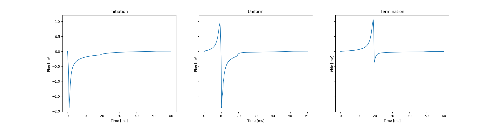
../../_images/unipolar_electrograms_ini_uni_term.png

Fig. 96 Visualization of recovered extracellular potentials at sites of initiating propagation ( $\phi_{\rm 0}$ in fig-tutorial-ecg B), uniform undisturbed propagation ( $\phi_{\rm 1}$ in fig-tutorial-ecg B) and terminating (or colliding) propagation ( $\phi_{\rm 2}$ in fig-tutorial-ecg B).

Activation spread in terms of transmembrane voltage $V_{\rm m}$ and extracellular potential $\phi_{\rm e}$ are shown in Fig. 97.

Fig. 97 Action potential propagation is elicited at the endocardial apical edge of the wedge. The spread of activation and repolarization is shown in terms of extracellular potential $\phi_{\rm e}$ and transmembrane voltage $V_{\rm m}$ . Field points at which extracellular potentials were recovered are shown in the right panel.

Experiments

Experiment exp01 (central endocardial activation (monodomain) with ecg recovery)

In a first step we omit a bath and use a monodomain as a source model. Extracellular potentials are computed using the $\phi_{\rm e}$ recovery technique. Propagation is initiated at the center of the endocardial surface as if activated by a Purkinje fascicle. Only 60 ms of activation are computed as we are only interested in the depolarization complex. Details on the CARPentry-specific definition of this method are found in the manual.

./run.py --sourceModel monodomain --duration 60 --visualize

In this case the extracellular potentials at the sites of stimulus delivery (vertex 0, initiating propagation), in the mid-myocardium (vertex 1, undisturbed uniform propagation) and at the epicardial surface (vertex 2, terminating propagation) shall be examined.

Experiment exp02 (apical endocardial activation (monodomain) with ecg recovery)

In experiment exp02 we shift the stimulus towards the apical edge of the wedge at the endocardium. The observation sites for recovering $\phi_{\rm e}$ remain the same, but local activation patterns underneath the recording electrodes are changed. This is reflected in the waveforms of the unipolar extracellular electrograms. Total activation time in this case is longer, we pick a larger duration therefore to allow for the entire wedge being activated.

./run.py --ab-stim-location apex --sourceModel monodomain --duration 100 --visualize

Experiment exp03 (apical endocardial activation (pseudo-bidomain) with ecg recovery, small bath)

We repeat exp02 using a pseudo-bidomain source model. This allows the comparison between extracellular potentials computed by the bidomain method with those computed by the recovery method. We start with a very small bath size of only 1 mm.

./run.py --ab-stim-location apex --sourceModel pseudo_bidomain --bath 1.0 --duration 60 --visualize

Experiment exp04 (apical endocardial activation (pseudo-bidomain) with ecg recovery, larger bath)

We repeat exp03 using a larger bath of 20 mm width to examine how bath size effects extracellular potential waveforms, their magnitude and differences between bidomain and recovery potentials.

./run.py --ab-stim-location apex --sourceModel pseudo_bidomain --bath 20.0 --duration 60 --visualize

Experiment exp05 (apical endocardial activation (monodomain) with ecg recovery, repolarization)

We repeat exp02, but run for longer to observe unipolar electrograms during repolarization.

./run.py --ab-stim-location apex --sourceModel monodomain --duration 400 --visualize

In this case it is of interest to examine so-called transmural ECGs, that is, the difference between unipolar electrograms recorded from endocardial and epicardial surfaces. The recovered unipolar ECG traces are stored in the file phie_recovery.igb in igb format in the respective output directories. We use :ref`igbextract <igbextract>` to compute the differences from the igb file and store the output in a text file for easier visualization. For this end we run:

./run.py --tmECG simID

where simID is the name of the output directory for which we want to compute the transmural ECG. The computed transmural ECG can be visualized, for instance, with gnuplot.

References

[1]	Bishop MJ, Plank G., Representing cardiac bidomain bath-loading effects by an augmented monodomain approach: application to complex ventricular models., IEEE Trans Biomed Eng 58(4):1066-75, 2011. [Pubmed] [PMC]

[2]	Bishop MJ, Plank G. Bidomain ECG simulations using an augmented monodomain model for the cardiac source. IEEE Trans Biomed Eng 58(4):1066-75, 2011. [Pubmed] [PMC]

[3]	Boukens B, Sulkin MS, Gloschat CR, Ng FS, Vigmond EJ, Efimov IR. Transmural APD gradient synchronizes repolarization in the human left ventricular wall. Cardiovasc Res 108(1):188-96, 2015. [Pubmed] [PMC]