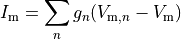
Tissue Scale
Model Equations
Discrete Representation
At a microscopic level cardiac tissue is a discrete structure
which is composed of myocytes interconnected
To understand activity at very fine resolutions, a discrete approach can be used where each cell is explicitly represented.
Ionic models of cells are connected to neighbouring cells with connectivity defined to represent actual tissue structure.
Gap junctions, providing the electrical coupling between cells, are depicted as ohmic resistances with the net cellular
membrane current,  , given as
(7)
where  is the neighbourhood of cells connected by gap junctions,
 is the gap junctional conductance between the cell under consideration and neighbour
which has a transmembrane voltage
is the gap junctional conductance between the cell under consideration and neighbour
which has a transmembrane voltage  .
A positive value of will lead to cellular depolarization
which can trigger an action potential if strong enough.
This equation can be combined with Eqn.~ref{eqn:Imdef} to determine the time course of the voltage.
.
A positive value of will lead to cellular depolarization
which can trigger an action potential if strong enough.
This equation can be combined with Eqn.~ref{eqn:Imdef} to determine the time course of the voltage.
Homogenization
The number of myocytes in the human heart is estimated to be in the range 2–3 billion. As such, this makes explicitly representing every cell computationally intractable. Instead of a discrete representation of individual cells, cardiac tissue is represented as a continuum in which properties are averaged over space. Homogenization is the process of determining a homogeneous material property which best replicates behaviour of the heterogeneous domain. Homogenized cardiac domain properties must be derived by taking into account myoplasmic properties, cellular structure, connectivity and orientation changes. The process assumes that properties and structure are the same in the subdomain being homogenized, allowing an average representation to be used.
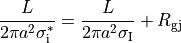
When determining homogenized conductivity values which encompass several myocytes,
there are two components to consider, one for the resistance of the cytoplasm, and one for the resistance of the gap junctions.
This is easily computed for the case of connected cylinders.
Considering the cylinders to have radius  and length
  with cytoplasmic conductivity
  and a gap junction resistance between cells of
  , we find the
homogenized conductivity
, we find the
homogenized conductivity  from the following equation:
(8)
The value of is itself homogenized
since cytoplasm has a conductivity close to that of sea water (1 S/m), but
the presence of organelles restrict the conduction path to decrease the effective conductivity.
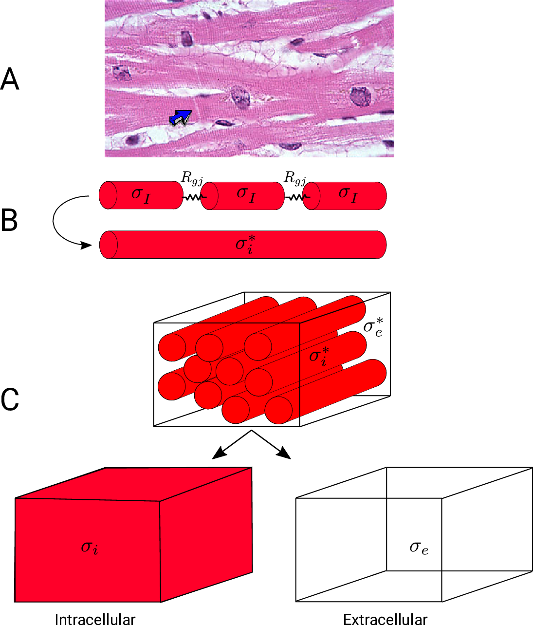
Fig. 41 A: Histological section of cardiac tissue. Nuclei are seen as purple ovals.
Junctions between cells are visible and oone is highlighted by the blue arrow.
B: Discrete myocytes with intracellular conductivity
are represented as cylinders, connected by gap junctions of resistance  ,
and form a syncytium with an equivalent conductivity, .
C: In the bidomain representation, tissue is composed of myocytes surrounded by an extracellular space.
After homogenization, the original volume is considered as two coincident domains,
each with homogenized properties.
,
and form a syncytium with an equivalent conductivity, .
C: In the bidomain representation, tissue is composed of myocytes surrounded by an extracellular space.
After homogenization, the original volume is considered as two coincident domains,
each with homogenized properties.
A further homogenization is required for mathematical approaches which treat intracellular and extracellular spaces to be continuous and everywhere within the cardiac tissue. These approaches consider each point to be in both spaces which is physically impossible. In effect, both domains are rescaled to fill the entire domain. Continuing the example of myocytes as cylinders packed in a volume, the effective conductivity in the longitudinal direction becomes
(9)
where  is the portion of the surface area of a plane orthogonal to the longitudinal axis
which is intracellular space.
Parameter values used in simulations may be quite different
from experimentally measured specific material properties due to homogenization.
is the portion of the surface area of a plane orthogonal to the longitudinal axis
which is intracellular space.
Parameter values used in simulations may be quite different
from experimentally measured specific material properties due to homogenization.
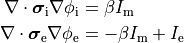
Bidomain Equation
Two domains are preserved in the formulation, the extracellular or interstitial space comprising the volume outside of and between the cells, and the intracellular space within myocytes. The membrane separates the intracellular from interstitial space. Due to the high degree of coupling, the intracellular space is considered a functional syncytium. The bidomain equations result from assuming that intracellular and extracellular domains exist everywhere, and that current flows between them by crossing the separating membrane, resulting in the following equations:
(10)
where  and
and  are the electrical potential and homogenized conductivity
in the domain
are the electrical potential and homogenized conductivity
in the domain  respectively, where
  is
is  or
or  for intracellular or extracellular.
The conductivity tensors describe the orthotropic eigendirections of the tissue at a given location,
for intracellular or extracellular.
The conductivity tensors describe the orthotropic eigendirections of the tissue at a given location,  ,
and are constructed as
,
and are constructed as
(11)
where  ,
,  and
and  are conductivities of the domain
along the local eigenaxes,
are conductivities of the domain
along the local eigenaxes,  , along the prevailing myocyte orientation referred to as fiber orientation,
perpendicular to the fiber orientation but within a sheet,
, along the prevailing myocyte orientation referred to as fiber orientation,
perpendicular to the fiber orientation but within a sheet,  , and the sheet normal direction,
  .
.
(12)
is the transmembrane voltage;
 is the surface area of membrane contained within a unit volume;
 is an extracellular current density, specified on a per volume basis,
which serves as a stimulus to initiate propagation;
is an extracellular current density, specified on a per volume basis,
which serves as a stimulus to initiate propagation;
At tissue boundaries, no-flux boundary conditions are imposed on  and
and  , i.e.,
(13)
holds. In those cases where cardiac tissue is surrounded by a conductive medium, such as blood in the ventricular cavities or a perfusing saline solution, an additional Poisson equation has to be solved
(14)
where  is the isotropic conductivity of the conductive medium and
 is the stimulation current injected into the conductive medium.
In this case, no flux boundary conditions are assumed at the boundaries of
the conductive medium, whereas continuity of the normal component of the
extracellular current and continuity of are enforced at the
tissue-bath interface. That is,
is the stimulation current injected into the conductive medium.
In this case, no flux boundary conditions are assumed at the boundaries of
the conductive medium, whereas continuity of the normal component of the
extracellular current and continuity of are enforced at the
tissue-bath interface. That is,
(15)
The no-flux boundary condition for along the tissue-bath interface remains unchanged
as the intracellular space is sealed there.
Equations (ref{eq:bidm_i}-ref{eq:bidm_e}) are referred to as the parabolic-parabolic form
of the bidomain equations, however, the majority of solution schemes is based
on the elliptic-parabolic form which is found by adding Eqs.~eqref{eq:bidm_i} and eqref{eq:bidm_e}
and replacing is by  .
This yields
.
This yields
(16)![\begin{eqnarray}
\left[
\begin{array}{c}
{ -\nabla \cdot \left( \boldsymbol{\sigma}_{\mathrm i} + \boldsymbol{\sigma}_{\mathrm e} \right) \nabla \phi_{\mathrm e} } \\
{ -\nabla \cdot \sigma_{\mathrm b} \nabla \phi_{\mathrm e} }
\end{array}
\right] &=&
\left[
\begin{array}{c}
{ \nabla \cdot \boldsymbol{\sigma}_{i} \nabla V_{\mathrm m} } \\
{ I_{\mathrm e} }
\end{array}
\right] \nonumber \\
-\left( \nabla \cdot \boldsymbol{\sigma}_{\mathrm i} \nabla V_{\mathrm m}
+\nabla \cdot \boldsymbol{\sigma}_{\mathrm i} \nabla \phi_{\mathrm e} \right) &=&
-\beta C_{\mathrm m} \frac{\partial V_{\mathrm m}}{\partial t} - \beta \left( I_{\mathrm {ion}} - I_{\mathrm {tr}} \right), \nonumber
\end{eqnarray}](../_images/math/bdc1a8f8ca7141943e3a0d6fac9acea34045a24a.png)
where  and , the quantities of primary concern, are retained as
the independent variables. Note that Eq.~eqref{equ:Elliptic} treats the bath
as an an extension of the interstitial space.
and , the quantities of primary concern, are retained as
the independent variables. Note that Eq.~eqref{equ:Elliptic} treats the bath
as an an extension of the interstitial space.
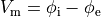
Monodomain Equation
A computationally less costly monodomain model can be derived from the bidomain model under the assumption
that intracellular and interstitial conductivity tensors can be related by
 .
In this scenario Eq.~eqref{eq:bidm_e} can be neglected
and the intracellular conductivity tensor in Eq.
.
In this scenario Eq.~eqref{eq:bidm_e} can be neglected
and the intracellular conductivity tensor in Eq. eq-Parabolic is replaced by the harmonic mean tensor,
 ,
,
(17)
That is, the monodomain equation is given by
(18)
where  is a transmembrane stimulus current,
a current which is introduced in the intracellular space and immediately removed from the extracellular space.
In this case, monodomain and bidomain formulations are equivalent in the sense
that both models yield the same conduction velocities along the principal axes
which, in turn, results in very similar activation patterns.
Minor deviations are expected when wavefronts are propagating in any other directions
which results in slightly different activation patterns.
is a transmembrane stimulus current,
a current which is introduced in the intracellular space and immediately removed from the extracellular space.
In this case, monodomain and bidomain formulations are equivalent in the sense
that both models yield the same conduction velocities along the principal axes
which, in turn, results in very similar activation patterns.
Minor deviations are expected when wavefronts are propagating in any other directions
which results in slightly different activation patterns.
This formulation has the advantage that it is computationally an order of magnitude of faster to solve than the bidomain formulation.
Though the equal anisotropy assumption is known to not hold, the approximation is reasonably accurate in situations
where extracellular fields are not imposed, which precludes its use for defibrillation studies.
Nevertheless, extracellular potentials can be recovered from the monodomain solution through the following:
(19)
Numerical details on discretization and solution of the bidomain equations were given previously in several studies [1] [2] [3].
Eikonal Model
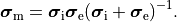
Fig. 42 Shown is the solution of the eikonal curvature equation,  ,
(right panel) in a finite element mesh of the left ventricle (left top)
with anisotropic conduction properties (left bottom, streamlines indicate direction of fastest propagation).
,
(right panel) in a finite element mesh of the left ventricle (left top)
with anisotropic conduction properties (left bottom, streamlines indicate direction of fastest propagation).
Reaction-Eikonal Model
TBA
Electrical Stimulation
Basically, cardiac tissue can be stimulated either by changing the electrical potential
or by injection/withdrawal of currents.
In both cases stimulation can be applied in the intracellular domain,  ,
or in the extracellular domain,
,
or in the extracellular domain,  .
Mathematically, voltage stimuli correspond to Dirichlet boundary conditions
whereas current stimuli are implemented either as Neumann boundary condition
or, alternatively, as volume sources.
The choice of stimulation procedure should be based on the experimental conditions to be modelled
and the electronic circuitry used in the voltage/current source.
If stimulation is mediated via controlled injection of currents the current stimulation methods is preferible,
otherwise if voltage sources are used the voltage stimulation method should be used.
A special case is the stimulation with a transmembrane current
where current is injected in one domain and withdrawn in the other domain at the exact same location.
Thus the stimulus itself does not set up a primary extracellular field as there is no current path
between injecting and withdrawing electrode.
An introduction to using electrical stimulation in CARPentry is given in the
Extracellular Stimulation Tutorial.
.
Mathematically, voltage stimuli correspond to Dirichlet boundary conditions
whereas current stimuli are implemented either as Neumann boundary condition
or, alternatively, as volume sources.
The choice of stimulation procedure should be based on the experimental conditions to be modelled
and the electronic circuitry used in the voltage/current source.
If stimulation is mediated via controlled injection of currents the current stimulation methods is preferible,
otherwise if voltage sources are used the voltage stimulation method should be used.
A special case is the stimulation with a transmembrane current
where current is injected in one domain and withdrawn in the other domain at the exact same location.
Thus the stimulus itself does not set up a primary extracellular field as there is no current path
between injecting and withdrawing electrode.
An introduction to using electrical stimulation in CARPentry is given in the
Extracellular Stimulation Tutorial.
Extracellular Voltage Stimulation
Mathematically, intracellular voltage stimulation is easily feasible,
but since this is of very limited practical relevance support for this type of stimulation is not implemented.
Voltage stimulation is therefore always applied in the extracellular domain  .
This is achieved by applying Dirichlet boundary conditions in
which directly alter extracellular potentials.
If we consider the bidomain equation governing the extracellular potential field
.
This is achieved by applying Dirichlet boundary conditions in
which directly alter extracellular potentials.
If we consider the bidomain equation governing the extracellular potential field
(20)
or in the elliptic-parabolic cast given by
(21)
extracellular voltage stimulatin is achieved
by enforcing the extracellular potential  to follow a given time course,
i.e.the prescribed stimulus pulse shape, over the entire electrode surface,
to follow a given time course,
i.e.the prescribed stimulus pulse shape, over the entire electrode surface, 
(22)
or, alternatively, also a spatial variation of extracellular potentials  is possible, that is,
In practice, voltage stimulation is performed with voltage sources. Voltage sources have two terminals which impose a potential relative to a reference usually referred to as ground (GND). Often one terminal is grounded, i.e.connected to a zero potential, whereas the other terminal prescribes the time course of the chosen pulse shape. Many other variations are also possible, but not all will be discussed. In the following we restrict ourselves to configurations which are realized typically in stimulation circuits.
Extracellular voltage stimulation with GND
This is the default setup for modeling extracellular voltage stimulation
where one terminal of the voltage sources is used
to prescribe the time course of the extracellular potential at one electrode,
and enforce a zero potential at the corresponding electrode.
If the enforced potentials are positive, that is  holds,
the positive terminal acts as an anode and the grounded terminal acts as a cathode.
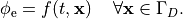
Such a configuration sets up an electric stimulation circuit as shown in Fig. 43.
On theoretical grounds, there is no necessity for using a ground electrode in this case
as a unique solution for the elliptic problem can be found by using one Dirichlet boundary conditions,
that is, using the electrode prescribing the stimulus pulse would suffice.
However, such a setup cannot be realized with an electric circuit and as such
it is unlikely to be suitable for matching a given experimental scenario.
holds,
the positive terminal acts as an anode and the grounded terminal acts as a cathode.
Such a configuration sets up an electric stimulation circuit as shown in Fig. 43.
On theoretical grounds, there is no necessity for using a ground electrode in this case
as a unique solution for the elliptic problem can be found by using one Dirichlet boundary conditions,
that is, using the electrode prescribing the stimulus pulse would suffice.
However, such a setup cannot be realized with an electric circuit and as such
it is unlikely to be suitable for matching a given experimental scenario.
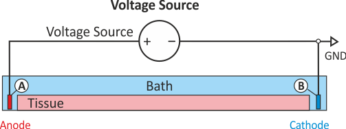
Fig. 43 Standard setup for extracellular voltage stimulation.
The positive terminal of the voltage source acts as an anode
by prescribing the time course of extracellular potentials .
The grounded electrode connected with the negative terminal of the voltage source acts as a cathode.
Symmetric extracellular stimulation with GND
The extracellular potential distribution  induced by the standard setup for extracellular voltage stimulation is not symmetric.
Under various circumstances it may be convenient to enforce an extracellular electric field
which is symmetric with regard to the two electrodes. Such a potential distribution can be enforced
using two electrodes of exactly opposite polarity and an additional ground
which then the zero potential isoline to run through the location of the grounding electrode.
This setup is shown in Fig. 44.
Configuration details for this setup are found XXX.
induced by the standard setup for extracellular voltage stimulation is not symmetric.
Under various circumstances it may be convenient to enforce an extracellular electric field
which is symmetric with regard to the two electrodes. Such a potential distribution can be enforced
using two electrodes of exactly opposite polarity and an additional ground
which then the zero potential isoline to run through the location of the grounding electrode.
This setup is shown in Fig. 44.
Configuration details for this setup are found XXX.
Fig. 44 Setup for generating a symmetric extracellular potential field. Electrodes A and B impose the exact same time course of , but with inverted signs. The location of the GND electrode determines the location of the zero potential isoline.
Open versus closed circuit stimulation
Depending on a given hardware, a switch may or may not interrupt the circuit after pulse delivery. If a switch remains closed for the entire simulation the potential at both electrodes are governed by the potentials of the terminals of the voltage source. Typically, the potential at both terminals will be zero after the pulse delivery, that is, both electrodes act as GND. This may not always be desired. If a switch interrupts the circuit after delivery the potential at one terminal is allowed to float whereas the other terminal will act as ground. An illustration of the difference between the two modes is given in Fig. 45.
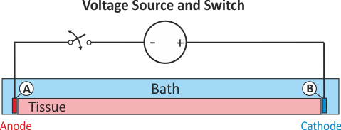
Fig. 45 Extracellular voltage stimulus with a switched terminal to interrupt the circuit after stimulation. In contrast to the standard setup for extracellular voltage stimulation the potential at electrode A is not clamped to a prescribed potential after the end of the pulse delivery, the potential there is allowed to float freely then.
Extracellular current stimulation
In many cases tissue is stimulated by injecting current through a current source. Modelingwise current stimulation is simpler to implement as there is no need for manipulating the left hand side of the equation system. Mathematically, current injection is modelled either as a Neumann boundary condition given as
(23)
or, alternatively, as a volmetric current source given as
(24)
where  is the volumetric current density.
While there are FEM-theoretical advantages of using a Neumann approach,
in terms of ease of implementation volumetric sources are more flexible and easier to handle.
A Neumann approach injects current through the surface of an electrode into the surrounding domain.
This is straight forward to implement when electrodes are located at the boundary of the extracellular domain
.
However, in many scenarios this is not the case, for instance, when modeling current injection into the blood pool of the RV
using a RV coil electrode of an implanted device.
In this case elements enclosed by the surface of the Neumann electrode should be removed.
The use of volumetric sources is simpler in this regard.
Electrodes can be located at arbitrary locations. The downside of volumetric sources is
that this method is not entirely mesh independent (current is injected via the FEM hat functions
and the total volume therefore varies therefore due to variability in the surface representation).
CARPentry implements volumetric sources, Neumann current sources are not implemented.
In those cases where mesh resolution dependence is unacceptable the total current to be injected can be prescribed
which is used for internal scaling of current density such that the prescribed total current is injected
indepdently of mesh resolution.
is the volumetric current density.
While there are FEM-theoretical advantages of using a Neumann approach,
in terms of ease of implementation volumetric sources are more flexible and easier to handle.
A Neumann approach injects current through the surface of an electrode into the surrounding domain.
This is straight forward to implement when electrodes are located at the boundary of the extracellular domain
.
However, in many scenarios this is not the case, for instance, when modeling current injection into the blood pool of the RV
using a RV coil electrode of an implanted device.
In this case elements enclosed by the surface of the Neumann electrode should be removed.
The use of volumetric sources is simpler in this regard.
Electrodes can be located at arbitrary locations. The downside of volumetric sources is
that this method is not entirely mesh independent (current is injected via the FEM hat functions
and the total volume therefore varies therefore due to variability in the surface representation).
CARPentry implements volumetric sources, Neumann current sources are not implemented.
In those cases where mesh resolution dependence is unacceptable the total current to be injected can be prescribed
which is used for internal scaling of current density such that the prescribed total current is injected
indepdently of mesh resolution.
It should be noted that the elliptic PDE as given in Eq. (21)
which has to be solved to find the extracellular potential distribution  is a pure Neumann problem and as such is singular.
That is, the solution can only be determined up to a given constant
as the Nullspace of a scalar Neumann problem comprises all constant functions.
Without using a Dirichlet boundary condition the problem cannot be solved therefore
unless an additional equation is used to constrain the solution in a unique way.
An often used constraint is to enforce the average potential in the domain to be zero,
that is
is a pure Neumann problem and as such is singular.
That is, the solution can only be determined up to a given constant
as the Nullspace of a scalar Neumann problem comprises all constant functions.
Without using a Dirichlet boundary condition the problem cannot be solved therefore
unless an additional equation is used to constrain the solution in a unique way.
An often used constraint is to enforce the average potential in the domain to be zero,
that is
(25)
Such constraints can be imposed with various stabilization techniques.
Extracellular current stimulation with GND
The standard setup for extracellular current stimulation comprises an electrode for current injection
combined with a ground electrode.
The ground electrode enforces a homogeneous Dirichlet boundary
thus rendering the problem non-singular and solvable without any additional constraints.
As shown in Fig. 46, assuming the current source delivers a positive current pulse
current is being injected in electrode A thus lifting the extracellular potential there.
The increase in drives the transmembrane voltage towards more negative
values, thus electrode A hyperpolarizes tissue in its adjacency and acts therefore as an anodal stimulus.
Electrode B is grounded. Any current injected in A is automatically collected electrode B
without the need of explicitly withdrawing current there.
As current is withdrawn at electrode B, is being lowered there
which drives towards more positive values.
Thus electrode B depolarizes tissue in its adjacency and acts therefore as a cathodal stimulus.
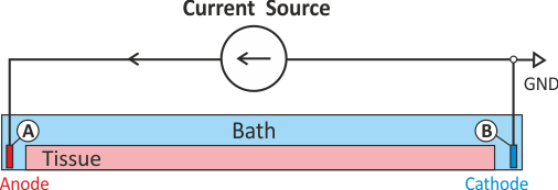
Fig. 46 Shown is the standard setup for current stimulation. Current is injected through electrode A which acts as an anode hyperpolarizing tissue in its adjacency. Conversely, electrode B is used to withdraw current acting as a cathodal stimulus which depolarizes tissue in its adjacency.
Extracellular symmetric current stimulation with diffuse GND
Similar to the scenario described above, the standard setup for extracellular current stimulation does not generate a symmetric potential field. However, a symmetric potential field can be setup by using two current electrodes, for instance, electrode A is used for injection and electrode B for withdrawing currents. However, in this case an additional difficulty arises stemming from the fact that we attempt to solve a pure Neumann problem. There are a two things to keep in mind:
When solving a pure Neumann problem one has to comply with the compatibility condition which boils down to the fact that the sum of all currents injected and withdrawn must balance out to zero. If we integrate over Eqs we obtain
(26)
Using Gauss’ diverence theorem we obtain the compatibility condition
(27)
essentially meaning that all extracellular stimulus currents must add up to zero.
A pure Neumann problem can be solved without a Dirichlet condition by resorting to solver techniques which deal with the Nullspace of the problem. Typically, a condition such as Eq. (25) is enforced. This can be considered to be a diffuse floating ground (see Fig. Fig. 47).
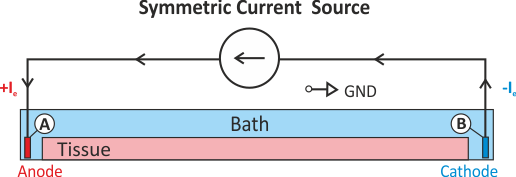
Fig. 47 Shown is a stimulation setup using injection of extracellular currents which induces a symmetric extracellular potential field. Note that a pure Neumann problem is solved here. A diffuse ground is used to render the problem solvable which boils down to imposing the additional constraint that the mean extracellular potential
is zero (see Eq. (25)).A setup with two current electrodes can be augmented with an additional reference electrode. In this case the compatibility condition does not need to be enforced. However, failure to balance the currents turns the ground electrode into an anode or cathode as any exess current will be collected by the ground electrode. Such a setup is shown in Fig. 48.
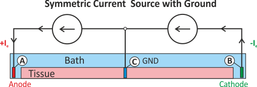
Fig. 48 Extracellular current injection with additional grounding electrode.
Definition of Electrical Stimuli
A complete definition of a stimulus comprises four components, the definition of electrode geometry, pulse shape, protocol and the physical nature of the pulse delivered (current or voltage). Stimuli are defined using the keyword stimulus[] where stimulus[] is an array of structures. The individual fields of the structure are defined in the following.
Geometry definition: Electrode geometries can be defined in two ways, indirectly by specifying a volume within which all mesh nodes are considered then to be part of this electrode, or, explicitly, by providing a vertex file containing the indices of all nodes to be stimulated.
The default definition is based on a block by specifying the lower left bottom corner and the lengths of the block along the Cartesian axes.
field type description name String Identifier for electrode used for output (optional) zd Float z-dimension of electrode volume yd Float y-dimension of electrode volume xd Float x-dimension of electrode volume z0 Float lower z-ordinate of electrode volume y0 Float lower y-ordinate of electrode volume x0 Float lower z-ordinate of electrode volume ctr_def flag if set, block limits are [ x0 - xd/2 x0 + xd/2], otherwise limits are [ x0 x0 + xd] etc Alternatively, other types of region than blocks are available such as spheres, cylinders or, the most general case, list of finite elements. See the definition of tag regions for details. Electrodes can be defined then by assigning the index of a tag region to the geometry field:
field type description geometry int Index of region pre-defined in tag region array tagreg[] An explicit definition of electrodes is also possible by providing a file holding all the mesh indices. A format definition of vertex files is given.
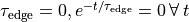
field type description vtx_file String File holding all nodal indices making up the electrode Pulse shape definition: By default, the pulse shape is defined as a monophasic pulse of square-like shape of a certain duration and strength. There are two time constants, one,
 , governs the leading and trailing edges of the pulse,
and one,
, governs the leading and trailing edges of the pulse,
and one,  , governs the plateau phase.
By default, these time constants are set to yield essentially a square-like pulse shape,
but can be easily adjusted to generate truncated exponential-like
pulses (see Fig. 49 for details).
Biphasic shapes are specified by two additional parameters,
the duration of the first part of the pulse relative to the duration of the entire pulse
(specified with
, governs the plateau phase.
By default, these time constants are set to yield essentially a square-like pulse shape,
but can be easily adjusted to generate truncated exponential-like
pulses (see Fig. 49 for details).
Biphasic shapes are specified by two additional parameters,
the duration of the first part of the pulse relative to the duration of the entire pulse
(specified with ![d1 \in (0,1]](../_images/math/c91efb130d56f4f71a7a667de63eb2eac4f20a19.png) ),
and the strength of the second part of the pulse relative to the strength of the first part,
),
and the strength of the second part of the pulse relative to the strength of the first part,
![s2 \in [0,1]](../_images/math/f630ea1c8b315ab3fea0bc9a1b3ab8c651ec492c.png) ).
The time constants for rising phases and plateau are the same for both polarities.
).
The time constants for rising phases and plateau are the same for both polarities.field type description s2 float strength relative to first part of biphasic pulse strength float amplitude of current ![[\mu A/cm^2]](../_images/math/c4bcd2abcc30af0d226484def126538135a622a7.png) or voltage
or voltage ![[mV]](../_images/math/afc8be4f1dc08ea0b1035ea02d14da386071b975.png)
total_current flag current strength is a total and not density d1 float duration of first part of biphasic pulse relative to total duration tau_edge float time constant for pulse edges tau_plateau float time constant for plateau bias float constant added to pulse duration float stimulus to be on pulse_file string Pulse file defining waveform 
balance int electrode with which to balance this electrode data_file string stimulus type-dependent data file An electrode balances another electrode be providing the same waveform as specified Electrode but of opposite polarity. For extracellular current injection, the strength takes into account Element sizes so that total current exiting one electrode enters the balanced electrode.
Mathematically, the pulses,
 , are defined:
(28)
![\begin{align}
P(t) & = B + \begin{cases}
S \left(1-e^{-t/\tau_{\mathrm {edge}}}\right) e^{-t/\tau_{\mathrm plateau}} & t\in [0,t'] \\
S_2 \left(1-e^{-(t-t')/\tau_{\mathrm edge}}\right) e^{-(t-t')/\tau_{\mathrm plateau}} & t\in (t',t''] \\
P(t'')e^{-(t-t'')/\tau_{edge}} & t \in(t'',D]
\end{cases} \nonumber
\end{align}](../_images/math/26bbb0f92e8d7fde0ef825ec1a91cafa90cf1d7f.png)
where
(29)
where
 is the specified strength,
  is the specified duration,
and
is the specified duration,
and  is the bias.
Note that for a monophasic pulse,
is the bias.
Note that for a monophasic pulse,  so that
  and only the top and bottom expressions are evaluated in Eq. (28)}.
Note the following:
and only the top and bottom expressions are evaluated in Eq. (28)}.
Note the following:- If
 .
. - To get an exponentially rising pulse, set
 negative.
 - To get an identically constant value, set
 and
and  .
.
Fig. 49 Top panels show the effect of parameters controlling the time constants of leading and falling edge
 ,
and the effect of the plateau time constant
,
and the effect of the plateau time constant  on a monophasic pulse.
Bottom panels show the effect of the duration ratio d1 and the strength ratio s2r
between the two phases of a biphasic stimulation pulse.
on a monophasic pulse.
Bottom panels show the effect of the duration ratio d1 and the strength ratio s2r
between the two phases of a biphasic stimulation pulse.- If
Stimulation source definition: The field stimtype field of the stimulus structure defines the physics of the actual source used for stimulating and, to some degree, also the wiring of the electric stimulation circuit. The following types of stimulation sources are supported:
field type value description stimtype short 0 transmembrane current 1 extracellular current 2 extracellular voltage (unswitched) 3 extracellular ground 4 intracellular current (unused) 5 extracellular voltage (switched) 6-7 unused 8 prescribed takeoff (see Reaction-Eikonal Model) 9 transmembrane voltage clamp Pacing protocol definition: The stimulus sequence is defined as a train of pulses. The number of pulses, the time interval between the pulses (pacing cycle length or basic cycle length) and the instant when first pulse is triggered defines the sequence in a unique manner. The following fields are used for the protocol definition:
field type description start float time at which stimulus sequence begins duration float duration of entire stimulus sequence npls int number of pulses forming the sequence (default is 1) bcl float basic cycle length for repetitive stimulation (npls > 1)
Electrical Tissue Properties
In CARPentry active and passive electrical tissue properties are assigned on a per region basis.
Regions are defined for a given properties as a set of tags (see Region Definition).
In cardiac electrophysiology simulations two distinct mechanisms are provided,
imp_region for the assignment of active electrophysiological properties,
that is, the assignment of models of cellular dynamics along with various specializations,
and gregion for the assignment of passive tissue properties
which govern subthreshold behavior and electrotonic features such as the space constant,  ,
but also influence suprathreshold phenomena such as conduction velocity and the spatial extent of depolarization wavefronts.
,
but also influence suprathreshold phenomena such as conduction velocity and the spatial extent of depolarization wavefronts.
Active Electrophysiological Properties
The number of regions is specified by num_regions.
Each region is preceded by imp_region[Int].
By default, elements are assigned {imp_region[0].
The following fields may be assigned:
| Variable | Type | Description |
|---|---|---|
| name | String | Region identification |
| num_IDs | Int | number of tags in the element file which belong to this regions |
| ID[Int] | Int * | array of the element tags belonging to the region |
| im | String | ionic model for this region. LIMPET specification |
| im_param | String | A comma separated list of parameters modifying the ionic model. These modifications are of the form param[=|*|/|+|-] float [%]. See the LIMPET library documentation for more details. |
| im_sv_dumps | String | comma separated list of state variables to dump from this IMP |
| im_sv_init | String | A file containing the initial values for variables’ statelabel{imsvdump} |
| plugins | String | comma separated list of plug-ins to use with the ionic model |
| plug_param | String | A colon separated list of comma separated lists specifying the plug-in parameters to modify. These are specified in the same order as the plug-ins are defined. |
| plug_sv_dumps | String | A colon list of comma separated lists specifying the state variables to dump for the plug-ins. Again, order must correspond to the order in which the plug-ins were specified. |
| cellSurfVolRatio | Float | If the ionic model does not specify the cellular surface to volume ratio, use this |
| volFrac | Float | fraction of tissue volume occupied by the cells |
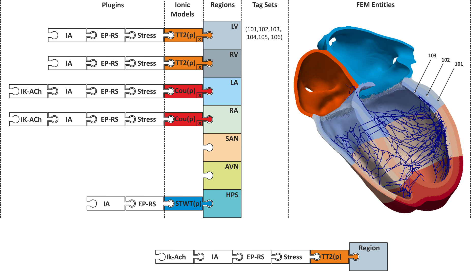
Fig. 50 Conceptual view on defining regions of different electrophysiological properties.
A region of similiar electrophysiological properties is an imp_region.
Each region is defined based on a set of tags which refer to finite element entities,
typically nodes or elements. Each imp_region is assigned exactly one model of cellular dynamics.
The model is parameterized with a set of parameters,  , which are constant over the entire imp_region.
If necessary, parameters can also vary as a function of space, ,
using the ion_adjustment mechanism.
Each ionic model can be augmented dynamically with a number of plug-ins (see augmentation).
, which are constant over the entire imp_region.
If necessary, parameters can also vary as a function of space, ,
using the ion_adjustment mechanism.
Each ionic model can be augmented dynamically with a number of plug-ins (see augmentation).
Passive Electrophysiological Properties
Similarly, different conductivities may be assigned to different elements.
The number of conductivities is specified with num_gregions.
The conductivity regions are specified by gregion[Int].
with each element initially assigned to gregion[0] by default.
The following fields specify a conductivity region:
| Variable | Type | Description |
|---|---|---|
| name | String | Region identification |
| num_IDs | Int | number of tags in the element file which belong to this regions |
| ID[Int] | Int * | array of the element tags belonging to the region |
| g_et | Float | extracellular transverse conductivity |
| g_it | Float | intracellular transverse conductivity |
| g_el | Float | extracellular longitudinal conductivity |
| g_il | Float | intracellular longitudinal conductivity |
| g_en | Float | extracellular sheet normal conductivity |
| g_in | Float | intracellular sheet normal conductivity |
| g_bath | Float | isotropic bath conductivity |
| g_mult | Float | multiplicator for conductivity scaling of a gregion |
where  are conductivities in the intracellular domain along the axes
 ,
,  are the respective conductivities in the extracellular domain
and
are the respective conductivities in the extracellular domain
and  is an isotropic conductivity assigned to elements in this regions marked as bath.
Bath elements in a region which are marked to be anisotropic use the values.
is an isotropic conductivity assigned to elements in this regions marked as bath.
Bath elements in a region which are marked to be anisotropic use the values.
Discrimination between isotropic bath and anisotropic bath, that is, anisotropic non-myocardium as it would be appropriate for skeletal muscles, occurs when reading in a mesh. The difference between these two cases manifests in the element and fiber files. An isotropic bath element is described as
Element                   Fiber
ID [Node Indices] Tag     l
...
Tt  0 1 144 1226   2      0.0 0.0 0.0
...
That is, these elements are identified as having a zero fiber orientation vector
whereas anisotropic bath elements do have a preferred fiber vector, optionally also a sheet vector,
but the Tag in the element file is negative:
Element                   Fiber
ID [Node Indices] Tag     l
...
Tt  0 1 144 1226  -2      1.0 0.0 0.0
...
Electrical Mapping
Measuring Reference Time Markers
The main purpose here is to detect at which instants in time
nodes are activated in the tissue. These instants are usually referred to
as local activation times. Experimentally, this is done usually
using extracellular signals, as input,
but transmembrane voltages can also be used, for instance,
when glass micro-electrodes are used (which would actually measure )
or in optical mapping experiments where  (see Sec. Optical Mapping is measured which is considered a surrogate for .
The implementation of this feature is actually more general,
it is an event detector that records the instants when the selected event type occurs.
Local activation detection in the extracellular signals usually relies on
detecting the minimum of the derivative of , i.e.  .
One could also detect the maximum of the derivative of , or,
the crossing of the action potential with a given threshold
which has to be chosen larger than the threshold for sodium activation.
That is, with one picks the maximum of
.
One could also detect the maximum of the derivative of , or,
the crossing of the action potential with a given threshold
which has to be chosen larger than the threshold for sodium activation.
That is, with one picks the maximum of  or when crosses the prescribed threshold with a positive slope.
Equally, one could look for crossing of with a negative slope
to detect repolarisation events. The basic idea is outlined in Fig. 51.
or when crosses the prescribed threshold with a positive slope.
Equally, one could look for crossing of with a negative slope
to detect repolarisation events. The basic idea is outlined in Fig. 51.
There can be num_LATs measurements and activation
can be defined in terms of a threshold or a derivative.
The activation measurements are named lats[Int].
with the following fields:
| field | type | description |
|---|---|---|
| measurand | Int | what to measure. 0=voltage, 1=extracellular potential |
| all | Int | If set, will output all activations as they occur. If zero, only the first activation of each vertex will be output. When all points are activated, one file with all the LATs will be written. |
| method | Int | How to determine activation. If method==0, use the
time at which the threshold was crossed. If method==1,
use the time of maximum derivative. |
| mode | Flag | If method==0, look for threshold crossing
with a negative slope (positive slope is default),
if method==1, look for minimum derivative instead of maximum |
| threshold | Float | The threshold value for determining activation.
If method==0, this is the threshold for detecting
activation, if method==1 the threshold is used
to exclude small peaks in the derivative which are not considered
to be due to local activation. |
| ID | Wfile | output file name |
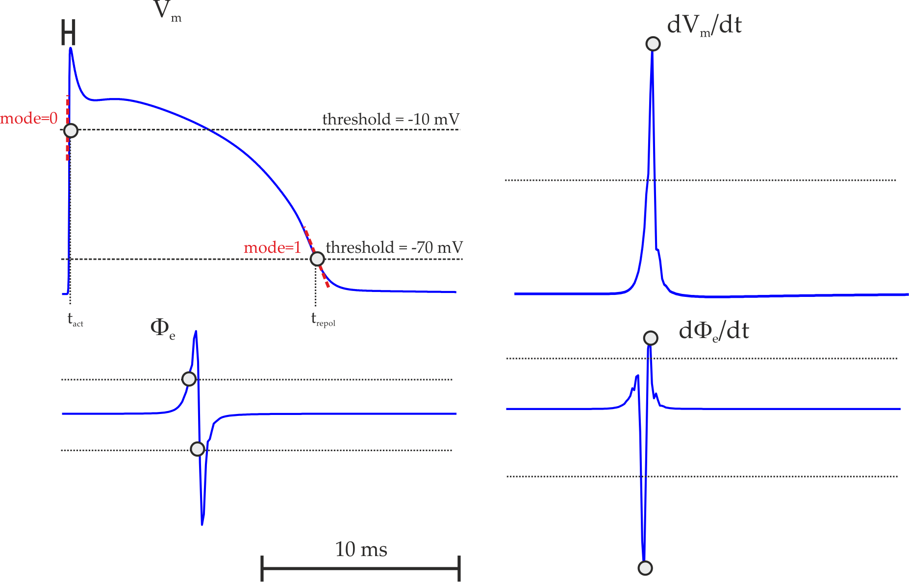
Fig. 51 Illustration of using the lat detection feature:
a) With measurand ,
using method==0, threshold  and
and mode==0,
all positive slope intersections of with the given threshold are detected.
In this case the instant of local activation,  is detected.
Using threshold
is detected.
Using threshold  and
and mode==1 the negative slope intersections are detected
which could be used in this case for detecting a reference marker for the instant of repolarisation,  .
b) Using
.
b) Using method==1 with measurand==0 ()
detects the peak derivative of .
Any peak derivatives below a chosen threshold are ignored.
c) Using threshold crossing detection on the extracellular signal ,
i.e. measurand==1.
d) Using peak derivative detection on the extracellular signal  ,
i.e.
,
i.e. measurand==1 and mode==1.
A tutorial on how to use these features is found in the Electrical Mapping Tutorial.
Measuring Conduction Velocities
Todo
explain carputils velocity script
Optical Mapping
To run an optical mapping experiment in post-processing,
both illuminating and emitting (or recording) surfaces need to be defined.
These are setup and defined like electrical electrodes being termed
illum_dbc and emission_dbc as they represent Dirichlet boundary conditions.
Like electrodes, they can be defined as a collection of points with boxes or with a list of vertices.
However, note that these points must lie on the surface of the tissue that you want to illuminate.
The illum_dbc.strength parameter should just be set to 1, although the magnitude does not really matter.
For now the em_dbc.strength is set to 0 on the surfaces from which you would like to compute the signal.
This is the most natural(ish) choice.
We assume that exactly just outside the tissue, there is no scattering, so photons zoom off to infinity,
thus leaving zero photon density just the other side of the boundary.
There is a more accurate mixed Neumann/Dirichlet boundary condition that could be implemented here,
but the differences are minimal (< 5 % between this and the more simple case of  .
In later versions, this other boundary condition may be added.
.
In later versions, this other boundary condition may be added.
| Variable | Type | Description | |
|---|---|---|---|
| num_illum_dbc | Int | Number of illumination Dirichlet boundary conditions | |
| num_emission_dbc | Int | Number of emmission Dirichlet boundary conditions | |
| optDT | Float | time step for optics in live mode,``0=no`` optics | |
| optics_mode | Int | Value | Description |
| 0 | Do not simulate optics | ||
| 1 | illuminate (for optogenetics simulations) | ||
| 2 | illumination and emission (optical maps) | ||
| phi_illum | Wfile | illumination photon source density,  |
|
| phi_em | Wfile | emission photon source density,  |
|
| w | Wfile | volumetric photon source density | |
| Vopt | Wfile | optical fluorescence signal | |
| mu_a_illum | Float | optical absorpitivity for illumination,  |
|
| Dopt_illum | Float | optical diffusitiviy for illumination,  |
|
| mu_a_em | Float | optical absorpitivity for emission,  |
|
| Dopt_em | Float | optical diffusitiviy for emission,  |
|
| illum_dbc | Optics_dbc* | boundary conditions for illumination | |
| emission_dbc | Optics_dbc* | boundary conditions for photon emission hline | |
Boundary Conditions
Like in the bidomain, on any surfaces which do not have a specific illumination or emission boundary condition imposed
we assume the standard zero flux condition of  .
This is ok for the sides of a slab, for example, which is being illuminated from its top side.
However, for the base of the slab this is not adequate,
and additional boundary conditions during both illumination and emission should be specified here.
Specifically,
.
This is ok for the sides of a slab, for example, which is being illuminated from its top side.
However, for the base of the slab this is not adequate,
and additional boundary conditions during both illumination and emission should be specified here.
Specifically,  should be defined on these surfaces.
This should only be worried about for thin slabs.
For anything thicker than
should be defined on these surfaces.
This should only be worried about for thin slabs.
For anything thicker than  or so, it does not really matter,
as the illuminating photon density will have decayed to almost zero here anyway
(although this should be adjusted for different illuminating wavelengths
which may penetrate deeper, as appropriate).
or so, it does not really matter,
as the illuminating photon density will have decayed to almost zero here anyway
(although this should be adjusted for different illuminating wavelengths
which may penetrate deeper, as appropriate).
| Variable | Type | Description |
|---|---|---|
| vtx_file | String | If specified, affected points given in this file |
| strength | Float | photon density on boundary |
| x0 | Float | lower z-ordinate of electrode volume |
| y0 | Float | lower y-ordinate of electrode volume |
| z0 | Float | lower z-ordinate of electrode volume |
| xd | Float | x-dimension of electrode volume |
| yd | Float | y-dimension of electrode volume |
| zd | Float | z-dimension of electrode volume |
| ctr_def | Flag | if set limits are [x0-xd x0+xd] etc, [x0 x0+xd] o.w. |
| geometry | Int | ID of dbc geometry definition |
| bctype | Short | 0=inomogeneous,1=homogeneous |
| dump_nodes | Flag | dump affected nodes in file |
Electrocardiogram
ECG signals can be either computed directly when running bidomain simulations or by using the integral solution of Poisson’s equation when running monodomain simulations given as
where are the potentials at a given field point,  ,
,
 is the source density at a given source point,
  ,
and
,
and  is the distance between source and field point.
A detailed description of the method and its limitation has been given in
(Bishop et al, IEEE Trans Biomed Eng 58(8), 2011),
is the distance between source and field point.
A detailed description of the method and its limitation has been given in
(Bishop et al, IEEE Trans Biomed Eng 58(8), 2011),
Bidomain simulations are the most appropriate approach when the heart is immersed in a volume conductor of limited size and the volume conductor can be represented. ECG recovery techniques are very well suited when the heart is immersed in an unbounded volume conductor. That is, ECG signals from a heart immersed in a torso can be approximated very well with a monodomain simulation using ECG recovery. On the other hand, ECG signals recorded at the surface of a Langendorff preparation are better approximated with a bidomain simulation when the heart is not immersed in a fluid bath. An alternative in this scenario is to use recovery method 3 where we use a monodomain simulation, but solve the elliptic PDE infrequently before outputting. Memorywise this simulation approach is equivalent to a bidomain simulations, in terms of execution speed the simulation is roughly equivalent to a monodomain simulation.
| field | type | description |
|---|---|---|
| phie_rec_ptf | string | file of recording sites (see Sref{sec:ptf} for format) |
| phie_recovery_file | Wfile | output file of ECG data |
| phie_rec_meth | Int | method to recover  |
A tutorial on how to use this ECG feature is found here.
References
| [1] | Plank G, Liebmann M, Weber dos Santos R, Vigmond EJ, Haase G. Algebraic multigrid preconditioner for the cardiac bidomain model, IEEE Trans Biomed Eng. 54(4):585-96, 2007. [PubMed] |
| [2] | Vigmond EJ, Weber dos Santos R, Prassl AJ, Deo M, Plank G. Solvers for the cardiac bidomain equations, Prog Biophys Mol Biol. 96(1-3):3-18, 2008. |PubMed| |
| [3] | Augustin CM, Neic A, Liebmann M, Prassl AJ, Niederer SA, Haase G, Plank G. Anatomically accurate high resolution modeling of human whole heart electromechanics: A strongly scalable algebraic multigrid solver method for nonlinear deformation, J Comput Phys. 305:622-646, 2016. [PubMed] |