`Electromechanical Single Cell Stretcher`

Module: tutorials.03_EM_single_cell.01_EM_coupling.run

Section author: Gernot Plank <gernot.plank@medunigraz.at> and Christoph Augustin <christoph.augustin@medunigraz.at>

Modeling EM at the cellular level

This tutorial introduces the basic steps of setting up EM simulations in an isolated myocytes. A more detailed account on modeling electro-mechanics at the cellular scale is given in the manual. For this sake an EP model of cellular dynamics must be paired with a myofilament model for generating active stresses. This is achieved by selecting an EP model of cellular dynamics and an active stress model as a plug-in. Setting up, initializing and testing of such myocyte-myofilament combinations is performed with our single cell tool bench. There are three coupling variants implemented which are suitable depending on a particular question to be addressed:

This setup aims to replicate single cell stretch experiments as they are performed with setups.

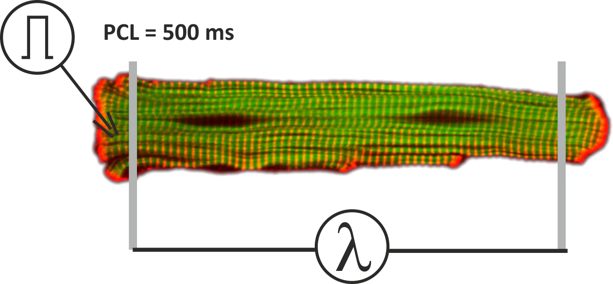
Fig. 120 Setup for single cell stretch experiments. The myocyte is activated with a supra-threshold stimulus current to initiate action potentials at a pacing cycle length of 500 ms. The length of the myocytes and thus the sarcomere stretch can be prescribed as a function of time.

Experimental Parameters

The following parameters are exposed to steer the experiment:

--experiment {active | passive}
                      Default is active. In the passive case any stimulation is turned off
                      and the myocyte remains quiescent. This can be used in the
                      strongly coupled case to observe the effect of step changes in length
                      upon EP states.

--EP                  pick human EP model (default is tt2)

--stress              pick stress model (default is tanh)

--stretch STRETCH     prescribe constant stretch over each cycle (default is 1.)

--init INIT           pick state variable initialization file (default is none)

--duration DURATION   pick duration of experiment (default is 500 ms)

--bcl BCL             pick basic cycle length (default is 500 ms)

--fs FS               provide trace file to prescribe fiber stretch (default is none)

--fsDot FSDOT         provide trace file to prescribe fiber stretch rate
                      (default is none)

--refH5 REFH5         pick h5 data set as reference for comparison (default is none)

Each experiment stores the state of myocyte and myofilament in the current directory in a file to be used as initial state vector in subsequent experiments.

Activation-based active stress model

Such models are suitable for being used in clinical EM modeling study as these models - owing to their small number of parameters and their fairly direct relation to clinically measurable parameters such as peak pressure, $\hat{P}$ or the maximum rate of rise of pressure, $dP/dt_{\mathrm {max}}$ - are easier to fit.

As an example we use the very simple tanh model. The model is based on activation times and constructed with exponential functions, it also accounts for length-dependent development of active tension. Our implementation of the tanh stress model is based on the PhD work of Andrew Crozier and has also been used in publications [1] [2].

The shape of the active stress transient is given by

$\begin{equation} T_{\rm a} = T_{\rm peak} \phi \tanh^2 \left( \frac{t_s}{\tau_{\rm c}} \right) \tanh^2 \left( \frac{t_\text{dur} - t_{\rm s}}{\tau_{\rm r}} \right) \text{for } 0< t_s < t_\text{dur} \nonumber \end{equation}$

with

$\begin{eqnarray} \phi &= \tanh (\text{ld} (\lambda - \lambda_{\rm 0})) \nonumber \\ \tau_{\rm c} &= \tau_{\rm c0} + \text{ld}_\text{up} (1 - \phi) \nonumber \\ t_{\rm s} &= t - t_\text{act} - t_\text{emd} \nonumber \end{eqnarray}$

with the following parameters:

Tab. 19 Parameters of the “tanh” stress model
Variable	Description
$t_{\rm s}$	onset of contraction
$\phi$	non-linear length-dependent function in which $\lambda$ is the fiber stretch
$\lambda_{\rm 0}$	fiber stretch below which no tension is generated anymore.
$t_{\mathrm {emd}}$	electro-mechanical delay
$T_{\mathrm {peak}}$	peak isometric tension
$t_{\mathrm dur}$	duration of tension generation
$\tau_{\mathrm {c}}$	time constant of contraction
$\tau_{\mathrm {c0}}$	baseline time constant of contraction $ld_{\mathrm {up}}$
$ld_{\mathrm {up}}$	length-dependence contraction time constant
$\tau_{\mathrm {r}}$	time constant of relaxation
$ld$	degree of length dependence
$ld_{\mathrm {on}}$	flag to turn on/off length-dependence of active stress generation local activation time
$t_{\mathrm {act}}$	which is automatically derived from the action potential, estimated as the instant of crossing the $V_{\rm m}$ threshold $V_{\mathrm{m,thresh}}$
$V_{\rm m,thresh}$	transmembrane voltage threshold used for detecting $t_{\mathrm {act}}$

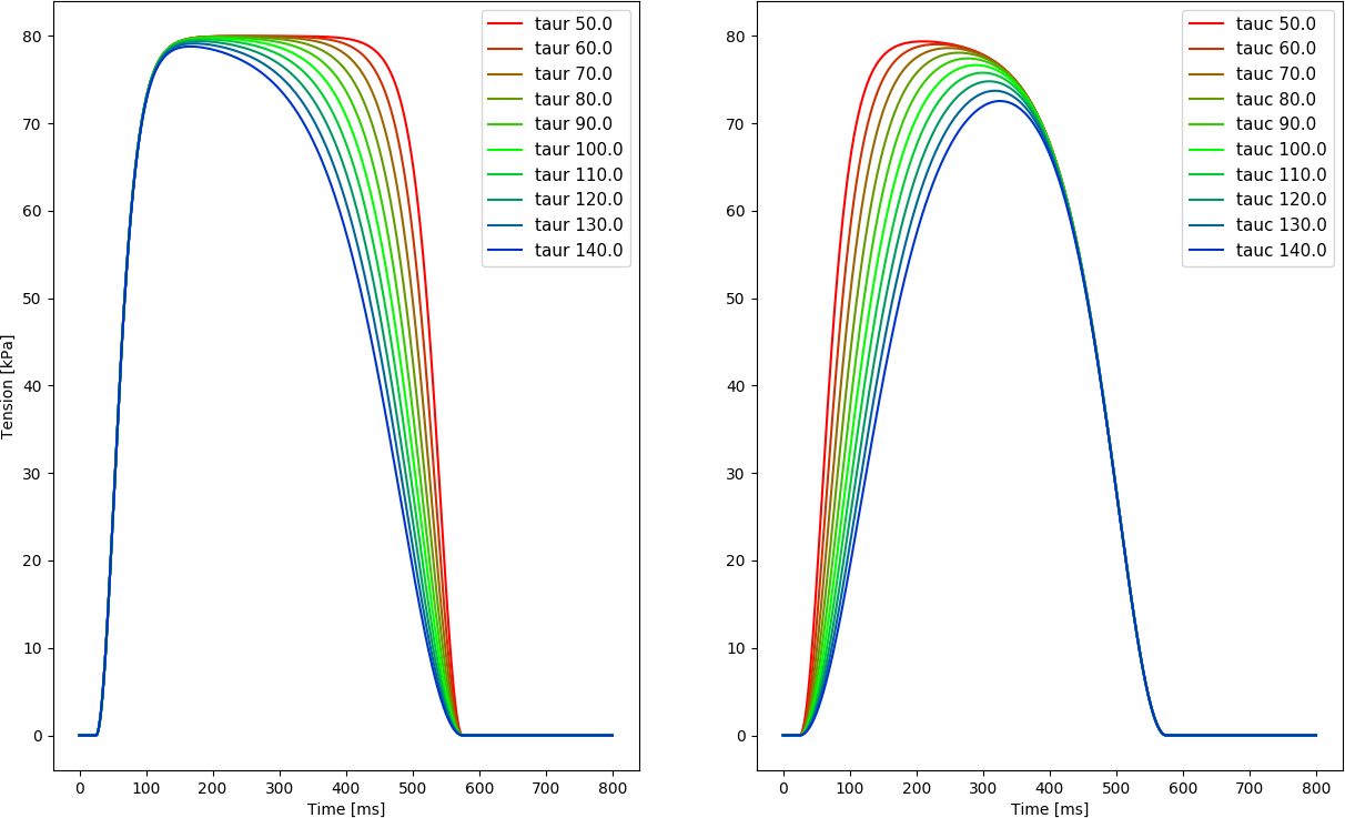
The effect of varying the time constants governing contraction $\tau_{\rm c}$ and relaxation, $\tau_{\rm r}$ , is shown below. Duration of the active stress transient was set to 550 ms in this case.

Experiment exp01

We start with coupling the Tanh stress model with the TT2 human myocyte model,

./run.py --EP tt2 --stress tanh --duration 2000 --bcl 500 --ID exp01 --visualize

Experiment exp02

As the TT2 is not at a limit cycle, we pace the model for 20 seconds

./run.py --EP tt2 --stress tanh --duration 20000 --bcl 500 --ID exp02 --visualize

In exp02 the states of myocyte and myofilament model are stored at the very end of the experiment at $t=20000 ms$ in the file exp01_tt2_tanh_bcl_500_ms_dur_20000_ms.sv.

Experiment exp03

Using the state of the myocyte stored in the file exp01_tt2_tanh_bcl_500_ms_dur_20000_ms.sv in exp02 we confirm now that your trajectories are close to a limit cycle for the given bcl and stretch we run

./run.py --EP tt2 --stress tanh --duration 1000 --bcl 500 --ID exp03 \
         --stretch 1.0 --init exp02_tt2_tanh_bcl_500_ms_dur_20000_ms.sv \
         --visualize

Observe that there is no significant difference between the traces for AP1 and AP2.

Experiment exp04

To ensure that length-dependence of active tension is working as expected re-run the experiment at a shorter cell length by setting the fiber stretch $\lambda=0.75$ and compare with the traces stored in exp03 in the file exp03_traces.h5.

./run.py --EP tt2 --stress tanh --duration 1000 --bcl 500 \
         --ID exp04 --stretch 0.75 --init exp02_tt2_tanh_bcl_500_ms_dur_20000_ms.sv \
         --refH5 exp03_traces.h5 --visualize

Experiment exp05

Re-run experiment exp04, but at a stretched cell length by setting the fiber stretch $\lambda=1.25$ and compare again with the traces stored in exp03 in the file exp03_traces.h5 at the reference cell stretch $\lambda=1.0$ .

./run.py --EP tt2 --stress tanh --duration 1000 --bcl 500 \
         --ID exp05 --stretch 1.25 --init exp02_tt2_tanh_bcl_500_ms_dur_20000_ms.sv \
         --refH5 exp03_traces.h5 --visualize

Weakly coupled Calcium-driven active stress model

As an example of a weakly coupled Calcium-driven active stress model due to Land et al for rat and rabbit myocytes [4] and for human myocytes [3]. Parameters used in this tutorial were derived from the study of Tondel et al [5].

Tab. 20 Parameters of the Land stress model
Variable	Description
$T_{\rm {ref}}$	Reference tension [kPa]
$Ca_{\rm {50ref}}$	Calcium sensitivity at resting sarcomere length
$TRPN_{\rm {50}}$	Troponin C sensitivity
$n_{\rm {TRPN}}$	Hill coefficient for cooperative binding of Calcium to Troponin C
$k_{\rm {TRPN}}$	Unbinding rate of Calcium from Troponin C
$n_{\rm {xb}}$	Hill coefficient for cooperative crossbridge action
$k_{\rm {xb}}$	scaling factor for the rate of crossbridge binding [ $\mathrm{ms}^{-1}$ ]
$\beta_{\rm {0}}$	magnitude of filament overlap effects
$\beta_{\rm {1}}$	magnitude of length-dependent activation effects

Experiment exp06

As before with the Tanh stress model, we pace the model for 20 seconds at a resting length of $\lambda=1.$ to arrive at a limit cycle.

./run.py --EP tt2 --stress land --duration 20000 --bcl 500 --ID exp06 --visualize

Observe that, unlike on the experiments with the Tanh stress model, tension transients vary over time as tension depends on Calcium. In exp06 the states of myocyte and myofilament model are stored at the very end of the experiment at 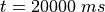$t=20000~ms$ in the file exp06_tt2_land_bcl_500_ms_dur_20000_ms.sv.

Experiment exp07

Using the state of the myocyte stored in the file exp06_tt2_land_bcl_500_ms_dur_20000_ms.sv in exp06 we confirm now that your trajectories are close to a limit cycle for the given bcl and stretch we run

./run.py --EP tt2 --stress land --duration 1000 --bcl 500 --ID exp07 \
         --stretch 1.0 --init exp06_tt2_land_bcl_500_ms_dur_20000_ms.sv \
         --visualize

Observe that there is no significant difference between the traces for AP1 and AP2.

Experiment exp08

To verify that the Land model in combination with the TT2 human ventricular myocyte models produces reasonable tensions over the physiological stretch range from $\lambda=0.75$ up to $\lambda=1.25$ we run two cycles at with a shortened myocyte $\lambda=0.75$ .

./run.py --EP tt2 --stress land --duration 1000 --bcl 500 \
         --ID exp08 --stretch 0.75 --init exp06_tt2_land_bcl_500_ms_dur_20000_ms.sv \
         --refH5 exp07_traces.h5 --visualize

Experiment exp09

Re-run experiment exp08, but at a stretched cell length by setting the fiber stretch $\lambda=1.25$ and compare again with the traces stored in exp07 in the file exp07_traces.h5 at the reference cell stretch $\lambda=1.0$ .

./run.py --EP tt2 --stress land --duration 1000 --bcl 500 \
         --ID exp09 --stretch 1.25 --init exp06_tt2_land_bcl_500_ms_dur_20000_ms.sv \
         --refH5 exp07_traces.h5 --visualize

Experiment exp10

Force development depends on both, length $\lambda$ and the velocity of length change $\dot{\lambda}$ . Increasing velocity $\dot{\lambda}$ lowers the force produced by a myocyte which produces the maximum force under isometric conditions, that is $\dot{\lambda} = 0$ . To illustrate these two effects indpendently we re-run exp09 with a dynamic sawtooth loading protocol shown in Fig. 121, but we keep the velocity at zero.

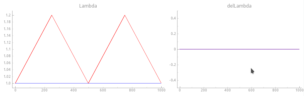
Fig. 121 Mechanical loading protocol applied to stretch the cell. Compared to the reference stretch experiment with $\lambda=1.0$ a sawtooth stretch function of time $\lambda(t)$ is applied. Velocity dependence is suppressed here by keeping $\dot{\lambda}(t)=0.$ . Blue traces show the loading protocol applied in exp09.

Note

This is artificial as we are altering $\lambda(t)$ and $\dot{\lambda}(t)$ independently.

./run.py --EP tt2 --stress land --duration 1000 --bcl 500 \
         --ID exp10 --init exp06_tt2_land_bcl_500_ms_dur_20000_ms.sv \
         --fs lambda_sawtooth_200ms.dat \
         --refH5 exp07_traces.h5 --visualize

Experiment exp11

In this experiment do not suppress velocity dependence anymore. The mechanical loading protocol applied is the same as in exp10, but with $\dot{\lambda}(t) \neq 0$ . The loading protocol is illustrated in Fig. 122.

Fig. 122 Mechanical loading protocol applied to stretch the cell. In this experimental protocol velocity-dependence of force generation is considered, that is, delLambda( $\dot{\lambda}(t)$ ) is indeed the derivative with respect to time of Lambda ( $\lambda(t)$ ). Blue traces show the loading protocol applied in exp10.

./run.py --EP tt2 --stress land --duration 1000 --bcl 500 \
         --ID exp11 --init exp06_tt2_land_bcl_500_ms_dur_20000_ms.sv \
         --fs lambda_sawtooth_200ms.dat --fsDot dlambda_sawtooth_200ms.dat \
         --refH5 exp10_traces.h5 --visualize

Strongly coupled Calcium-driven active stress model

In this set of experiments we couple the recent EP model of the human ventricular myocyte due to Grandi et al [6] (Grandi-Pasqualini-Bers GPB) with the active tension model due to Land et al [4] (Land-Niederer LN). Details on the implementation and parameterization of the coupling have been reported in detail in Augustin et al [9].

Briefly, to allow for strong coupling, i.e., to account for length effects on the cytosolic calcium transient, modifications were implemented to both the GPB and the LN model. The equation governing the binding of calcium to the low affinity regulatory sites on Troponin in the myofilament model (see Eq.~(114) in the Appendix of [6])

(39) $\begin{align} \frac{\mathrm{d}[\mathrm{TnC}_{\mathrm{L}}]}{\mathrm{d} t} = k_{\mathrm{on}_{\mathrm{TnC}_{\mathrm{L}}}}[\mathrm{Ca}_{\mathrm{i}}^{2+}] \left(\hat{B}_{\mathrm{TnC}_{\mathrm{L}}} -[\mathrm{TnC}_{\mathrm{L}}] \right) - k_{\mathrm{off}_{\mathrm{TnC}_{\mathrm{L}}}} [\mathrm{TnC}_{\mathrm{L}}] \nonumber \end{align}$

is replaced by the analogous Eq.~(1) of the LN active stress model [4], given as

(40) $\begin{align} \frac{\mathrm{d}\,\mathrm{TRPN}}{\mathrm{d} t} = k_{\mathrm{TRPN}} \left(\frac{[\mathrm{Ca}_{\mathrm{i}}^{2+}]} {[\mathrm{Ca}_{\mathrm{i}}^{2+}]_{\mathrm{T50}}(\lambda)} \right)^{n_\mathrm{TRPN}} \hspace{-2ex}\left(1 - \mathrm{TRPN}\right) - k_{\mathrm{TRPN}}\, \mathrm{TRPN}. \nonumber \end{align}$

In the combined GPB+LN model (39) is replaced by (40), scaled by the total buffer concentration $\hat{B}_{\mathrm{TnC}_{\mathrm{L}}}$ assumed to be 70 $\mu M/L$ in the GPB model. This scaling is necessary to correctly relate fractional occupancy, used by the LN myofilament model, with the concentration of Troponin bound calcium, used by the GPB model. Parameters of the GPB model were left unaltered whereas parameters of the LN model were adapted to give human myocardium tension transients when coupled to the GPB calcium transient [5].

In single cell experiments, both the unaltered GPB model and the combined GPB+LN model were paced at a cycle length of 500 ms for a duration of 60 seconds. In the combined GPB+LN model the stretch ratio was kept constant at $\lambda=1.0$ over the entire protocol. In both models, all state variable transients were plotted over the entire pacing experiment to ensure that the system had settled close to a stable limit cycle. The effect of the altered Troponin buffering equation in the GPB+LN model relative to the GPB model is illustrated in Fig. 123.

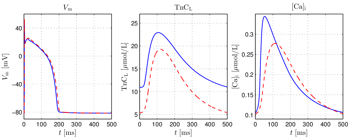
Fig. 123 Comparison of $V_{\mathrm{m}}$ , $\mathrm{TnC}_{\mathrm{L}}$ and $[\mathrm{Ca}_{\mathrm{i}}^{2+}]$ single cell traces between the GPB model (blue) and the GPB+LN model at steady state with $\lambda=1$ (red).

The effect of strong coupling in the GPB+LN model under fixed stretch conditions in the range $\lambda\in[1.0,1.2]$ , with the same pacing protocol, is illustrated in Fig. 124.

../../_images/gpb_strong_length_dep_Cai.png

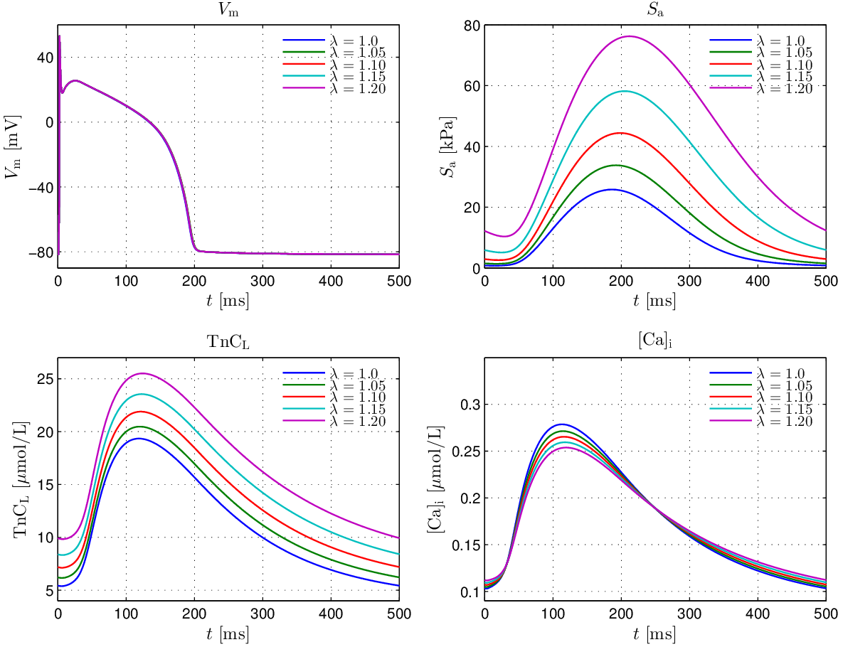
Fig. 124 Steady state traces of $V_{\mathrm{m}}$ , isometric tension, $\mathrm{TnC}_{\mathrm{L}}$ and $[\mathrm{Ca}_{\mathrm{i}}^{2+}]$ in a single cell pacing experiment under varying stretch ratios.

Experiment exp12 (pace to limit cycle)

As before, we pace the model for 20 seconds at a resting length of $\lambda=1.$ to arrive at a limit cycle.

./run.py --EP gpb_land --duration 20000 --bcl 1000 --ID exp12  \
         --no-filter --visualize

Experiment exp13 (confirm limit cycle)

Using the state of the myocyte stored in the file exp12_gpb_land_bcl_1000_ms_dur_20000_ms.sv in exp12 we confirm now that your trajectories are close to a limit cycle for the given bcl and stretch we run

./run.py --EP gpb_land --duration 2000 --bcl 1000 --ID exp13 --stretch 1.0 \
         --init exp12_gpb_land_strongly_coupled_bcl_1000_ms_dur_20000_ms.sv \
         --visualize

Observe that there is no significant difference between the traces for AP1 and AP2.

Experiment exp14 (return to rest)

As this model is strongly coupled, mechanical loading influences EP in the myocyte. To observe MEF effects we leave the limit cycle and stop pacing for 2 seconds. That is, in this experiment we keep the myocyte quiescent, we do not deliver an electrical stimulus current, nor a mechanical stretch protocol and observe the return of trajectories to a resting state.

./run.py --experiment passive --EP gpb_land --duration 1000 --bcl 1000 \
         --ID exp14 --stretch 1.0 \
         --init exp12_gpb_land_strongly_coupled_bcl_1000_ms_dur_20000_ms.sv \
         --visualize

Experiment exp15 (stretch resting myocyte, velocity dependence off)

To observe the effect of cellular stretch upon EP we apply now mechanical loading protocols to the resting myocyte. As a reference case, we apply a step change in stretch of 20% and observe only length-dependent effects, that is, velocity-dependence is turned off. This is achieved with the loading protocol shown in Fig. 125.

../../_images/gpb-land-mef-ld-protocol.png

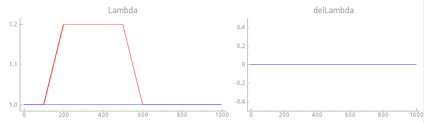
Fig. 125 Mechanical loading protocol applied to stretch the cell. Velocity dependence is turned off in this case by setting $\dot{\lambda}=0.0$ (delLambda).

./run.py --experiment passive --EP gpb_land --duration 1000 --bcl 1000 \
         --ID exp15 --init exp14_gpb_land_strongly_coupled_bcl_1000_ms_dur_1000_ms.sv \
         --fs lambda_step_tr_time_100ms.dat --visualize

Experiment exp16 (stretch resting myocyte, velocity dependence on, slower transition)

We repeat experiment exp15 now, but with velocity dependence enabled. First, we use a moderately fast step change by going from $\lambda=1.0$ to $\lambda=1.2$ in 100 ms and compare results with exp15 where velocity dependence was disabled. See Fig. 126.

../../_images/gpb-land-mef-ld-vd-slow-protocol.png

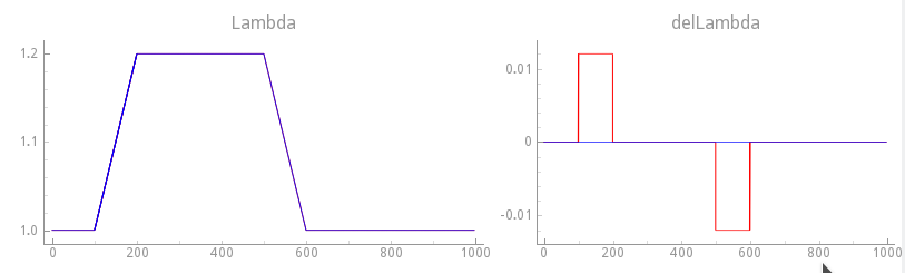
Fig. 126 Comparison of stretch protocols between exp15 where velocity dependence was disabled ( $\dot{\lambda}=0.0$ ) and with velocity-dependence enabled using a transition rate of the step change of 20% over 100 ms.

./run.py --experiment passive --EP gpb_land --duration 1000 --bcl 1000 \
         --ID exp16 --init exp14_gpb_land_strongly_coupled_bcl_1000_ms_dur_1000_ms.sv \
         --fs lambda_step_tr_time_100ms.dat --fsDot dlambda_step_tr_time_100ms.dat \
         --refH5 exp15_traces.h5 --visualize

Experiment exp17 (stretch resting myocyte, velocity dependence on, faster transition)

We repeat experiment exp16 now, but with velocity dependence enabled. We use a faster step change by going from $\lambda=1.0$ to $\lambda=1.2$ in only 10 msecs. See Fig. 127.

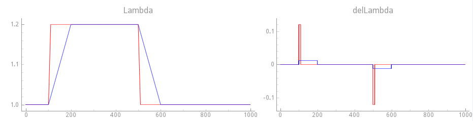
../../_images/gpb-land-mef-ld-vd-fast-protocol.png

Fig. 127 Comparison of stretch protocols between slow transition (100 ms) and fast transition (10 ms) step changes.

./run.py --experiment passive --EP gpb_land --duration 1000 --bcl 1000 \
         --ID exp17 --init exp14_gpb_land_strongly_coupled_bcl_1000_ms_dur_1000_ms.sv \
         --fs lambda_step_tr_time_10ms.dat --fsDot dlambda_step_tr_time_10ms.dat \
         --refH5 exp16_traces.h5 --visualize

Strongly coupled electro-mechanical human ventricular myocyte model with passive component

In this set last set of experiments we couple the recent EP model of the human ventricular myocyte due to Tomek et al [7] (Tomek-Rodriguez-O’Hara-Rudy ToR-ORd) with the active tension model due to Land et al [3] (Land-Niederer LN). Details on the implementation and parameterization of the coupling have been reported in Margara et al [8].

Experiment exp18 (pace to limit cycle)

As before, we pace the model for 20 seconds to arrive at a limit cycle.

./run.py --EP torord_landhumanstresswithpassive --duration 20000 \
         --bcl 1000 --ID exp18 --no-filter --visualize

Experiment exp19 (confirm limit cycle)

Using the state of the myocyte stored in the file exp18_torord_landhumanstresswithpassive_strongly_coupled_bcl_1000_ms_dur_20000_ms.sv in exp18 we confirm now that your trajectories are close to a limit cycle for the given bcl and stretch we run

./run.py --EP torord_landhumanstresswithpassive --duration 2000 \
         --bcl 1000 --ID exp19 \
         --init exp18_torord_landhumanstresswithpassive_strongly_coupled_bcl_1000_ms_dur_20000_ms.sv \
         --visualize

Observe that there is no significant difference between the traces for AP1 and AP2.

Experiment exp20 (return to rest)

Again, as this model is strongly coupled, mechanical loading influences EP in the myocyte. To observe MEF effects we leave the limit cycle and stop pacing for 2 seconds. That is, in this experiment we keep the myocyte quiescent, we do not deliver an electrical stimulus current, nor a mechanical stretch protocol and observe the return of trajectories to a resting state.

./run.py --experiment passive --EP torord_landhumanstresswithpassive \
         --duration 1000 --bcl 4000 --ID exp20 --visualize \
         --init exp18_torord_landhumanstresswithpassive_strongly_coupled_bcl_1000_ms_dur_20000_ms.sv

Literature

[1]	Niederer SA, Plank G, Chinchapatnam P, Ginks M, Lamata P, Rhode KS, Rinaldi CA, Razavi R, Smith NP. Length-dependent tension in the failing heart and the efficacy of cardiac resynchronization therapy, Cardiovasc Res 89(2):336-43, 2011. [PubMed] [Full Text]

[2]	Crozier A, Blazevic B, Lamata P, Plank G, Ginks M, Duckett S, Sohal M, Shetty A, Rinaldi CA, Razavi R, Smith NP, Niederer SA. The relative role of patient physiology and device optimisation in cardiac resynchronisation therapy: A computational modelling study, [PubMed] [Full Text]

[3]	(1, 2) Land S, Park-Holohan SJ, Smith NP, Dos Remedios CG, Kentish JC, Niederer SA. A model of cardiac contraction based on novel measurements of tension development in human cardiomyocytes, J Mol Cell Cardiol. 106:68-83, 2017. [PubMed]

[4]	(1, 2, 3) Land S, Niederer SA, Aronsen JM, Espe EK, Zhang L, Louch WE, Sjaastad I, Sejersted OM, Smith NP An analysis of deformation-dependent electromechanical coupling in the mouse heart, J Physiol 590(18):4553-69, 2012. [PubMed]

[5]	(1, 2) Tondel K, Land S, Niederer SA, Smith NP. Quantifying inter-species differences in contractile function through biophysical modelling, J Physiol 593(5):1083-111, 2015. [PubMed] [Full Text]

[6]	(1, 2) Grandi E, Pasqualini FS, Bers DM. A novel computational model of the human ventricular action potential and Ca transient, J Mol Cell Cardiol 48, 112-121, 2010. [PubMed] [Full Text]

[7]	Tomek J, Bueno-Orovio A, Rodriguez B. ToR-ORd-dynCl: an update of the ToR-ORd model of human ventricular cardiomyocyte with dynamic intracellular chloride, bioRxiv, 2020. [Full Text]

[8]	Margara F, Wang ZJ, Levrero-Florencio F, Santiago A, Vasquez M, Bueno-Orovio A, Rodriguez B. In-silico human electro-mechanical ventricular modelling and simulation for drug-induced pro-arrhythmia and inotropic risk assessment, Prog Biophys Mol Biol 159:58-74, 2021. [PubMed] [Full Text]

[9]

Augustin CM, Neic A, Liebmann M, Prassl AJ, Niederer SA, Haase G, Plank G. Anatomically accurate high resolution modeling of human whole heart electromechanics: A strongly scalable algebraic multigrid solver method for nonlinear deformation, J Comput Phys. 305:622-646, 2016. [PubMed ] [Full Text]