Unloading
Module: tutorials.04_EM_tissue.03_unloading.run
Section author: Matthias Gsell <matthias.gsell@medunigraz.at>
Calculate the unloaded reference geometry from a known mesh configuration under loading.
Introduction
Patient-specific models for numerical simulations of the cardiovascular system are mainly based on medical imaging techniques such as X-ray computed tomography (CT) or magnetic resonance imaging (MRI). But at the moment of the medical image acquisition, a physiological pressure load is present. When using the in vivo obtained patient-specific model, this model does not correspond to the unloaded configuration. Thus, we need a suitable algorithm to determine the unloaded configuration from the in vivo model and from the present physiological pressure.
Method
For our purpose, we use a backward displacement method described in [Bols2013] which is based
on a fixed-point iteration. Before we describe the method, we make some definitions. We denote
by  the stress free reference configuration which is yet
unknown. The first argument
the stress free reference configuration which is yet
unknown. The first argument  denotes the material coordinates and the second argument
 corresponds to stress ( which is zero ) of the unloaded configuration. A simple
forward computation leads to the equilibrium configuration
corresponds to stress ( which is zero ) of the unloaded configuration. A simple
forward computation leads to the equilibrium configuration  ,
with the coordinates of the deformed geometry
,
with the coordinates of the deformed geometry  and the second-prder stress tensor
 . This configuration results from a pressure load
  applied at the inner
surface of the undeformed configuration, i.e.
applied at the inner
surface of the undeformed configuration, i.e.
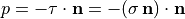
with the outer normal vector  , and
, and  at the outer surface.
See figure Fig. 135.
at the outer surface.
See figure Fig. 135.
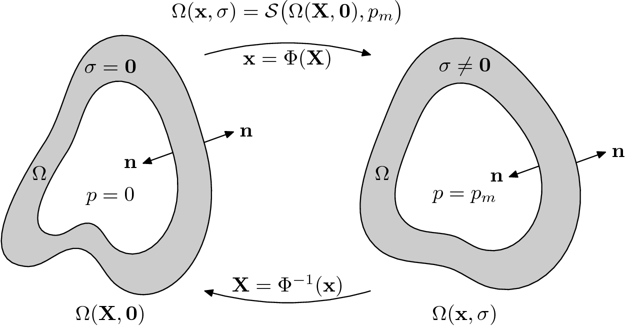
Fig. 135 Unloaded and loaded configuration.
We write
where  is an appropriate forward solver. The deformation is then defined
by the mapping
is an appropriate forward solver. The deformation is then defined
by the mapping  .
.
We denote the measured geometry and the measured pressure load by  and
and
 respectively. Then the backward problem is as follows.
Find the in vivo configuration  which is
unknown since just is known, and which is in equilibrium. Therefore, we
have to find the corresponding unloaded configuration such that
which is
unknown since just is known, and which is in equilibrium. Therefore, we
have to find the corresponding unloaded configuration such that

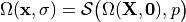
where  denotes the unknown unloaded reference geometry which can
be written as
denotes the unknown unloaded reference geometry which can
be written as 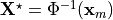 .
.
Algorithm
The backward displacement method then reads as follows.
![\intertext{\textbf{Input:} Measured state $\Omega_m^r = \Omega(\mathbf{x}_m, \mathbf{0})$ and pressure $p_m$} \\[-1.2cm]
& \line(1,0){330} \\[-0.5cm]
\intertext{Set initial stress free configuration $\Omega_1^r = \Omega(\mathbf{X}_1, \mathbf{0})$ with $\mathbf{X}_1 = \mathbf{x}_m$} \\[-1cm]
& i = 0 \\
& \textbf{while} \; (\text{error} > \varepsilon) \; \textbf{do} \\
& \qquad i = i + 1 \\
& \qquad \Omega_i^t = \Omega(\mathbf{x}_i, \mathbf{\sigma}_i) = \mathcal{S}\big(\Omega_i^r, p_m\big) \\
& \qquad \mathbf{U}_i = \mathbf{x}_i - \mathbf{X}_i \\
& \qquad \mathbf{X}_{i+1} = \mathbf{x}_m - \mathbf{U}_i \\
& \qquad \Omega_{i+1}^r = \Omega(\mathbf{X}_{i+1}, \mathbf{0}) \\
& \qquad \text{error} = error(\Omega_m^r, \Omega_i^t) \\
& \textbf{end do} \\
& \line(1,0){330} \\[-0.5cm]
\intertext{\textbf{Output:} Zero pressure geometry $\Omega(\mathbf{X}^{\star}, \mathbf{0})$ with $\mathbf{X}^{\star} = \mathbf{X}_i$} \\[-1.2cm]
\intertext{\phantom{\textbf{Output:}} In vivo stress tensor $\mathbf{\sigma}^{\star} = \mathbf{\sigma}_i$ } \\[-1.2cm]](../../_images/math/c37f9da81f4664d2b8af445da2cccb5120ef5197.png)
Usage
To run a simple ring example just run the command
./run.py --meshtype ring --pressure 4.0 --fast --visualize
where the parameter meshtype specifies the mesh and pressure is the
pressure to unload from. The visualize flag runs meshalyzer and shows
the result. For further information / help on the arguments and flags see below, to get the full
help run ./run.py --help.
  -h, --help                             show this help message and exit

  --pressure PRESSURE                    End diastolic pressure to unload from ( in kPa )
                                         (default: 1.5kPa for ring/ellipsoid, 5kPa for cube)

  --np NP                                number of processes

  --meshtype TYPE                        choose the mesh type,
                                         choices = {cube,ring,ellipsoid}

  --dimension DIMENSION                  choose the inner diameter of the mesh cavity, or the
                                         side length in the case of a cube ( in mm )

  --fast                                 set resolution and material (example specific) to
                                         fast-solving values

  --resolution RES                       set target mesh resolution ( in mm )

  --material TYPE                        choose the material model
                                         choices = {mooneyrivlin, linear, neohookean, holzapfelogden,
                                                    demiray, anisotropic, holzapfelarterial,
                                                    stvenantkirchhoff, guccione}

  --parameters PRM=VAL [PRM=VAL ...]     set material model parameters

MATERIAL PARAMETERS:
     mooneyrivlin { kappa, c_1, c_2 }
     linear { E, lmbda, mu, nu }
     neohookean { kappa, c }
     holzapfelogden { kappa, a, a_f, a_fs, a_s, b, b_f, b_fs, b_s }
     demiray { kappa, a, b }
     anisotropic { kappa, a_f, b_f, c }
     holzapfelarterial { kappa, c, k_1, k_2 }
     stvenantkirchhoff { lmbda, mu }
     guccione { kappa, b_f, b_fs, b_t, a }
Examples
In this section we want to present two examples to which the algorithm was applied. The black wireframe shows the initial geometry.
Fig. 136 Three dimensional ring.
Fig. 137 Three dimensional ellipsoid.
References
| [Bols2013] | Bols, J. and Degroote, J. and Trachet, B. and Verhegghe, B. and Segers, P. and Vierendeels, J., A computational method to assess the in vivo stresses and unloaded configuration of patient-specific blood vessels (2013), Journal of computational and Applied mathematics, Volume 246 |