Running A Simulation In carputils mode
carputils Overview
The increasing complexity of in silico experiments as they have become feasible over the past few years prompted for the development of a framework that simplifies the definition and execution of such experiments which become quickly intractable otherwise even for expert users. The major design goals were
- Encapsulate the technical complexity to enable users to perform experiments at a more abstract level
- Once built, limited technical expertise should be required to carry out in silico experiments, thus relieving users from undergoing months/years of training and thus save time to be spent on actual research
- Expose only steering parameters required for a given experiment
- Enable the easy sharing of experiments for collaborative research, re-use of used/published experiments or simply for the sake of remote debugging/advising
- Provide built-in capabilities for generating high quality documentation of experiments
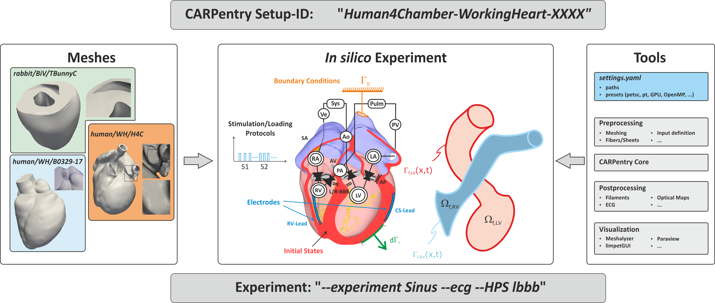
Fig. 5 Simplified definition of in silico experiments within the CARPentry modeling framework.
Discrete representations of hearts are stored in repositories from where they are loaded when needed.
Not only the meshes themselves, but also derived discrete entities such as element/vertex lists or
surfaces are stored there to be used for defining electrodes or boundary conditions.
The location of all tools for performing the experiments and for analyzing experimental data
are encapsulated in the python-based carputils package
which is also used to describe the experiment, that is, link the exposed input parameters
used to steer the experiment to create appropriate sets of commands
which are used to execute the experiment.
To share an experiment only the CARPentry experiment ID and the exact experimental protocol
are needed to be replicated elsewhere.
carputils is a Python package containing a lot of CARPentry-related
functionality and a framework for running CARPentry simulations and testing their
outputs en masse. Provided functionality includes:
- Scripting environment for designing complex in silico experiments
- Generation of CARP command line inputs with:
- Automatic adding of MPI launcher
- Debugger and profiler attachment
- Automatic batch script generation and submission with platform-specific hardware profiles
- Compact model setup using Python classes
- Efficient IO of common CARPentry file formats to numpy arrays
- Failure-compliant mass running of tests
- Automatic comparison of test results against reference solutions
Structure
The CARP examples framework encompasses a number of repositories, the purpose of which can be initially confusing. This section aims to explain the structure.
A typical installation might look like:
software
├── carputils
├── carp-examples
│   ├── benchmarks
│   └── devtests
├── carp-meshes
└── carp-reference
    ├── benchmarks
    └── devtests
carputils- A repository containing most of the Python functionality used in setting up
and postprocessing CARP simulations. The
binsubdirectory should be added to yourPATHenvironment variable, and the top level directory should be added to yourPYTHONPATH. On first run of an experiment, or when using the automatic clone script, thesettings.yamlfile will be generated, which must be tailored to your setup. carp-examples- This is a normal directory which contains 2 (or more) Python packages whose
modules define experiments. Each
run.pyscript in these packages runs an experiment. In fact, as long ascarputilsis set up correctly, you can move these run scripts anywhere on your system (along with any input files they depend on) and they will work, but in order to run regression tests they must be inside these packages andcarp-examplesmust be added to thePYTHONPATH. carp-meshes- This is an SVN repository containing meshes used by examples. As it is very
large, you may instead use the
--get-meshflag with run scripts to get only their needed meshes. Note that most run scripts generate meshes programmatically, in which case this is not needed. The location of this repository is set incarputils/settings.yamlwithMESH_DIR. carp-reference- These directories contain the reference solutions for regression tests. The
repositories under
carp-referencemust have the same name as those undercarp-examples. These repositories are only needed for running regression tests. The location ofcarp-referenceis set by theREGRESSION_REFsettings incarputils/settings.yaml
Note
The actual structure above need not be conformed to. It only matters that
carputils and carp-examples are in the PYTHONPATH,
carputils/bin is in the PATH, and carp-meshes and
carp-reference are at the locations specified in settings.yaml.
Other than that you can put them where you want.
Concepts
The following concepts are used in the carputils framework:
- sim
- A single CARP execution - consecutive, related runs are considered to be multiple sims
- job
- One or more related sims launched by a single execution of a carputils run script
- example
- A carputils run script, capable of launching a single job per execution, though different jobs can be launched by changing the command line arguments
- test
- A fixed (according to the command line arguments) run configuration of an example plus several checks to determine the accuracy of the output
- check
- A method to determine the accuracy of the output of a test - most commonly by comparing with a previous reference solution but also may be by comparison with an analytic solution and other custom methods
Generate HTML Page
This documentation is based on Sphinx and can be generated using the Makefile in the carputils/doc folder.
cd carputils/doc
make clean
make html
The html webpages are found then in the folder carputils/doc/build/html. To view, point your favorite browser to
firefox ${CARPUTILS_DIR}/doc/build/html/index.html
First Run
With the installation complete, you should be able to cd to a test
directory and run examples there with the run.py scripts. Run with:
./run.py
or:
python run.py
Add the --help or -h option to see a list of command line options and inputs
defined for this specific experiment.
The options shown by --help consist of four distinct sections,
optional arguments, execution options and experimental input arguments,
output arguments and debugging and profiling options.
usage: run.py [-h] [--np NP] [--tpp TPP] [--runtime HH:MM:SS]
              [--build {CPU,GPU}]
              [--flavor {petsc,boomeramg,parasails,pt,direct}]
              [--platform {desktop,archer,archer_intel,archer_camel,curie,medtronic,mephisto,smuc_f,smuc_t,smuc_i,vsc2,vsc3,wopr}]
              [--queue QUEUE] [--vectorized-fe VECTORIZED_FE] [--dry-run]
              [--CARP-opts CARP_OPTS] [--gdb [PROC [PROC ...]]]
              [--ddd [PROC [PROC ...]]] [--ddt] [--valgrind [OUTFILE]]
              [--valgrind-options [OPT=VAL [OPT=VAL ...]]] [--map]
              [--scalasca] [--ID ID] [--suffix SUFFIX]
              [--overwrite-behaviour {prompt,overwrite,delete,error}]
              [--silent] [--visualize] [--mech-element {P1-P1,P1-P0}]
              [--postprocess {phie,optic,activation,axial,filament,efield,mechanics}
                 [{phie,optic,activation,axial,filament,efield,mechanics} ...]]
              [--tend TEND] [--clean]

optional arguments:

  -h, --help            show this help message and exit
  --CARP-opts CARP_OPTS
                        arbitrary CARP options to append to command
  --mech-element {P1-P1,P1-P0}
                        CARP default mechanics finite element (default: P1-P0)
  --postprocess {phie,optic,activation,axial,filament,efield,mechanics} [{phie,optic,activation,axial,filament,efield,mechanics} ...]
                        postprocessing mode(s) to execute
  --tend TEND           Duration of simulation (ms)
  --clean               clean generated output files and directories

execution options:

  --np NP               number of processes
  --tpp TPP             threads per process
  --runtime HH:MM:SS    max job runtime
  --build {CPU,GPU}     CARP build to use (default: CPU)
  --flavor {petsc,boomeramg,parasails,pt,direct}
                        CARP flavor
  --platform {desktop,archer,archer_intel,archer_camel,curie,medtronic,mephisto,smuc_f,smuc_t,smuc_i,vsc2,vsc3,wopr}
                        pick a hardware profile from available platforms
  --queue QUEUE         select a queue to submit job to (batch systems only)
  --vectorized-fe VECTORIZED_FE
                        vectorized FE assembly (default: on with FEMLIB_CUDA,
                        off otherwise)
  --dry-run             show command line without running the test

debugging and profiling:

  --gdb [PROC [PROC ...]]
                        start (optionally specified) processes in gdb
  --ddd [PROC [PROC ...]]
                        start (optionally specified) processes in ddd
  --ddt                 start in Allinea ddt debugger
  --valgrind [OUTFILE]  start in valgrind mode, use in conjunction with --gdb
                        for interactive mode
  --valgrind-options [OPT=VAL [OPT=VAL ...]]
                        specify valgrind CLI options, without preceding '--'
                        (default: leak-check=full track-origins=yes)
  --map                 start using Allinea map profiler
  --scalasca            start in scalasca profiling mode

output options:

  --ID ID               manually specify the job ID (output directory)
  --suffix SUFFIX       add a suffix to the job ID (output directory)
  --overwrite-behaviour {prompt,overwrite,delete,error}
                        behaviour when output directory already exists
  --silent              toggle silent output
  --visualize           toggle test results visualisation
To understand how the command line of individual experiments is built
it may be insightful to inspect the command line assembled and executed by the script.
This is achieved by launching the run script with an additional --dry option.
For instance, running a simple experiment like
./run.py --visualize --dry
yields the following output (marked up with additional explanatory comments)
--------------------------------------------------------------------------------------------------------------------------------
                                     Launching CARP Simulation 2017-06-13_simple_20.0_pt_np8
--------------------------------------------------------------------------------------------------------------------------------

# pick launcher, core number and executable
mpiexec -n 8 /home/plank/src/carp-dcse-pt/bin/carp.debug.petsc.pt \
\
# feed in static parameter sets compiled in the par-file
  +F simple.par \
\
# provide petsc and pt solver settings for elliptic/parabolic PDE, mechanics PDE and Purkinje system
  +F /home/plank/src/carputils/carputils/resources/options/pt_ell_amg \
  +F /home/plank/src/carputils/carputils/resources/options/pt_para_amg \
  +F /home/plank/src/carputils/carputils/resources/options/pt_mech_amg \
  -ellip_options_file /home/plank/src/carputils/carputils/resources/options/pt_ell_amg \
  -parab_options_file /home/plank/src/carputils/carputils/resources/options/pt_para_amg \
  -purk_options_file /home/plank/src/carputils/carputils/resources/petsc_options/pastix_opts \
  -mechanics_options_file /home/plank/src/carputils/carputils/resources/options/pt_mech_amg \
  \
# pick numerical settings, toggle between pt or petsc, Purkinje always uses petsc
  -ellip_use_pt 1 \
  -parab_use_pt 1 \
  -purk_use_pt 0 \
  -mech_use_pt 1 \
  \
# simulation ID is the name of the output directory
  -simID 2017-06-13_simple_20.0_pt_np1 \
  \
# pick the mesh we use and define simulation duration
  -meshname meshes/2016-02-20_aTlJAwvpWB/block \
  -tend 20.0 \
  \
# define electrical stimulus
  -stimulus[0].x0 450.0 \
  -stimulus[0].xd 100.0 \
  -stimulus[0].y0 -300.0 \
  -stimulus[0].yd 600.0 \
  -stimulus[0].z0 -300.0 \
  -stimulus[0].zd 600.0 \
  \
# some extra output needed for visualization purposes
  -gridout_i 3 \
  -gridout_e 3

-------------------------------------------------------------------------------------------------------------------------------
                                     Launching Meshalyzer
-------------------------------------------------------------------------------------------------------------------------------

/home/plank/src/meshalyzer/meshalyzer 2017-06-13_simple_20.0_pt_np1/block_i \
                                      2017-06-13_simple_20.0_pt_np1/vm.igb.gz simple.mshz
It is always possible to change general global settings such as the solvers to be used or the target computing platform for which the command line is being assembled.
For instance, switching from the default flavor pt set in settings.yaml to flavor petsc is achieved by
./run.py --visualize --flavor petsc --dry
Compared to above, the numerical settings selection has changed
...
# whenever possible, we use petsc solvers now
-ellip_use_pt 0 \
-parab_use_pt 0 \
-purk_use_pt 0 \
-mech_use_pt 0 \
...
Setting a different default platform in the settings.yaml file or at the command line
through the --platform input parameter changes launcher and command line,
also generating a submission script if run on a cluster.
For instance, we can easily generate a submission script for the UK national supercomputer ARCHER
by adding the appropriate platform string
./run.py --np 532 --platform archer --runtime 00:30:00 --dry
which writes a submission script and, without the --dry option, would directly submit to the queuing system
Requested mesh already exists, skipping generation.
---------------------------------------------------------------------------------------------------------------------------
                                Batch Job Submission
---------------------------------------------------------------------------------------------------------------------------

qsub 2017-06-14_simple_20.0_pt_np528.pbs
with the generated submission script
#!/bin/bash --login
#PBS -N 2017-06-14_simp
#PBS -l select=22
#PBS -l walltime=00:30:00
#PBS -A e348

# Make sure any symbolic links are resolved to absolute path
export PBS_O_WORKDIR=$(readlink -f $PBS_O_WORKDIR)

# Change to the directory that the job was submitted from
# (remember this should be on the /work filesystem)
cd $PBS_O_WORKDIR

# Set the number of threads to 1
#   This prevents any system libraries from automatically
#   using threading.
export OMP_NUM_THREADS=1

################################################################################
# Summary

# Run script executed with options:
# --np 528 --platform archer --runtime 00:30:00 --dry

################################################################################
# Execute Simulation

mkdir -p 2017-06-14_simple_20.0_pt_np528

aprun -n 528 /compute/src/carp-dcse-pt/bin/carp.debug.petsc.pt \
  +F simple.par \
  +F /compute/src/carputils/carputils/resources/options/pt_ell_amg_large \
  +F /compute/src/carputils/carputils/resources/options/pt_para_amg_large \
  +F /compute/src/carputils/carputils/resources/options/pt_mech_amg_large \
  -ellip_use_pt 1 \
  -parab_use_pt 1 \
  -purk_use_pt 0 \
  -mech_use_pt 1 \
  -ellip_options_file /compute/src/carputils/carputils/resources/options/pt_ell_amg_large \
  -parab_options_file /compute/src/carputils/carputils/resources/options/pt_para_amg_large \
  -purk_options_file /compute/src/carputils/carputils/resources/petsc_options/pastix_opts \
  -mechanics_options_file /compute/src/carputils/carputils/resources/options/pt_mech_amg_large \
  -vectorized_fe 0 \
  -mech_finite_element 0 \
  -simID 2017-06-14_simple_20.0_pt_np528 \
  -meshname meshes/2015-12-04_qdHibkmous/block \
  -tend 20.0 \
  -stimulus[0].x0 450.0 \
  -stimulus[0].xd 100.0 \
  -stimulus[0].y0 -300.0 \
  -stimulus[0].yd 600.0 \
  -stimulus[0].z0 -300.0 \
  -stimulus[0].zd 600.0
Writing Examples/Tutorials
CARP example simulations are created using the carputils framework in a
standardised way that seeks to promote conciseness and familiarity to
developers. Writers of new examples are therefore advised to first look over
existing examples. Look in the directory hierarchy of the devtests or
benchmarks repositories - examples are the python source files conventionally
named run.py in directories whose name describes the main purpose of the
example.
Note
For a complete working example simulation, please look at the ‘simple bidomain’ example in the devtests repository (devtests/bidomain/simple), which can be copied and adapted to create new examples.
The carputils framework can be used by any python script on a machine where it
is installed - scripts do not need to be placed inside the devtests or
benchmarks repositories. The reasons to place them there is to share them
conveniently with others and for inclusion in the automatic testing system
carptests.
Anatomy of an Example
A CARP run script will contain at a minimum:
from carputils import tools

@tools.carpexample()
def run(args, job):
    # Generate CARP command line and run example
    pass # Placeholder

if __name__ == '__main__':
    run()
The script defines a run function which takes as its arguments a namespace
object containing the command line parameters (generated by the standard
library argparse module) and a Job object. The run
function should use the carputils.tools.carpexample() function decorator,
as shown, which generates the above arguments and completes some important pre-
and post-processing steps.
Many of the tasks of run scripts are common between examples, for example for
setting up the correct CARP command line options for a particular solver.
carputils therefore performs many of these common tasks automatically or by
providing convenience functions. Below is a more complete example:
"""
Description of the example.
"""

EXAMPLE_DESCRIPTIVE_NAME = 'Example of Feature X'
EXAMPLE_AUTHOR = 'Joe Bloggs <joe.bloggs@example.com>'

from datetime import date
from carputils import tools

def parser():
    # Generate the standard command line parser
    parser = tools.standard_parser()
    group  = parser.add_argument_group('experiment specific options')
    # Add an extra argument
    group.add_argument('--experiment',
                        default='bidomain',
                        choices=['bidomain', 'monodomain'])
    return parser

def jobID(args):
    today = date.today()
    ID = '{}_{}_{}_np{}'.format(today.isoformat(), args.experiment,
                                args.flv, args.np)
    return ID

@tools.carpexample(parser, jobID)
def run(args, job):

    # Generate general command line
    cmd = tools.carp_cmd('example.par')

    # Set output directory
    cmd += ['-simID', job.ID]

    # Add some example-specific command line options
    cmd += ['-bidomain', int(args.experiment == 'bidomain'),
            '-meshname', '/path/to/mesh']

    # Run example
    job.carp(cmd)

if __name__ == '__main__':
    run()
Example Breakdown
Below the various parts of the above example are explained.
carputils.tools.standard_parser() returns an ArgumentParser object
from the argparse module of the python standard library. You can then add
your own example-specific options in the manner shown. See
the argparse documentation
for information on how to add different types of command line option.
To make it easier to identify experiment specific options, an argument group is created and
arguments added directly to it.
This is optional but increases clarity.
def parser():
    # Generate the standard command line parser
    parser = tools.standard_parser()
    group  = parser.add_argument_group('experiment specific options')
    # Add an extra argument
    group.add_argument('--experiment',
                        default='bidomain',
                        choices=['bidomain', 'monodomain'])
    return parser
The jobID function generates an ID for the example when run. The ID is used
to name both the example output directory and the submitted job on batch
systems. The function takes the namespace object returned by the parser as an
argument and should return a string, ideally containing a timestamp as shown:
def jobID(args):
    today = date.today()
    ID = '{}_{}_{}_np{}'.format(today.isoformat(), args.experiment,
                                args.flv, args.np)
    return ID
The carputils.tools.carpexample() decorator takes the above parser and
jobID functions as arguments. It takes care of some important pre- and
post-processing steps and ensures the correct arguments are passed to the run
function at runtime:
@tools.carpexample(parser, jobID)
def run(args, job):
carputils.tools.carp_cmd() generates the initial command line for the
CARP executable, including the correct solver options for the current run
configuration the standard command line parser generated above. If you are
using a CARP parameter file, pass the name as an optional argument to
carp_cmd(), otherwise just call with no argument:
# Generate general command line
cmd = tools.carp_cmd('example.par')
The CARP command must always have a -simID argument set. When your example
runs CARP only once, this will be the ID attribute of the job object
passed to run, otherwise it should be a subdirectory:
# Set output directory
cmd += ['-simID', job.ID]
Your example should then add any additional command line arguments to the command list:
# Add some example-specific command line options
cmd += ['-bidomain', int(args.experiment == 'bidomain'),
        '-meshname', '/path/to/mesh']
Finally, use the carp method of the job object to execute the
simulation. The reason for this, rather than executing the command directly,
is that the job object takes care of additional preprocessing steps and
automatically generates batch scripts on HPC systems. To run shell commands
other than CARP, see the carputils.job.Job documentation.
# Run example
job.carp(cmd)
At the very end of your run script, add the below statements. This executes the run function when the file is executed directly:
if __name__ == '__main__':
    run()
Documenting Examples
Examples should be well commented, but should also start with a descriptive python docstring to serve as a starting point for new users. This should include:
- A description of the feature(s) the example tests.
- Relevant information about the problem setup (mesh, boundary conditions, etc.)
- The meaning of the command line arguments defined by the example, where this is not obvious.
The docstring must be at the top of the file, before any module imports but
after the script interpreter line, and is essentially a comment block started
and ended by triple quotes """:
#!/usr/bin/env python

"""
An example testing the ...
"""

EXAMPLE_DESCRIPTIVE_NAME = 'Example of Feature X'
EXAMPLE_AUTHOR = 'Joe Bloggs <joe.bloggs@example.com>'
The docstring should be followed by two variables as above.
EXAMPLE_DESCRIPTIVE_NAME should be a short descriptive name of the test to
be used as a title in the documentation, e.g. ‘Activation Time Computation’ or
‘Mechanical Unloading’. EXAMPLE_AUTHOR should be the name and email address
of the primary author(s) of the test in the format seen above. Multiple authors
are specified like:
EXAMPLE_AUTHOR = ('Joe Bloggs <joe.bloggs@example.com>,'
                  'Jane Bloggs <jane.bloggs@example.com> and'
                  'Max Mustermann <max.mustermann@beispiel.at>')
Formatting
The docstring is used to build the example documentation at https://carpentry.medunigraz.at/carputils/examples/, and can include reStructuredText formatting. Some key features are summarised below, but for a more comprehensive summary of the format please see the Sphinx webstie. It is important to bear in mind that indentation and blank lines have significance in rst format.
Headings are defined by underlining them with =, -, +,
~, with the order in which they are used indicating the nesting
level: |
Heading 1
=========

Heading 1.1
-----------

Heading 1.1.1
+++++++++++++

Heading 1.2
-----------
|
Python code highlighting is done by ending a paragraph with a double
colon :: followed by an indented block: |
Here is an example of a run function::

    def run(argv, outdir=None):
        for list in argv:
            print argv
|
Highlighting of other languages is done with a code-block
directive: |
.. code-block:: bash

    echo "some message" > file.txt
|
LaTeX-formatted maths may be inserted with the math environment
(info): |
.. math::

    (a + b)^2 = a^2 + 2ab + b^2

    (a - b)^2 = a^2 - 2ab + b^2
|
| or inline: | I really like the equation :math:`a^2 + b^2 = c^2`.
|
Images may be included, but must be stored in the doc/images
directory of carputils. The path used in the image directive must
then begin with /images to work correctly. |
.. image:: /images/ring_rigid_bc.png
|
carputils Mesh Generation
carputils provides extensive functionality for the automatic generation of meshes according to geometric shapes. This currently includes:
- 1D cable (
carputils.mesh.Cable) - 2D grid (
carputils.mesh.Grid) - Block/cuboid (
carputils.mesh.Block) - Ring/cylindrical shell (
carputils.mesh.Ring) - Ellipsoidal shell (
carputils.mesh.Ellipsoid)
The carputils.mesh module also provides some utility functions to be
used with the above classes. See the API documentation
for more information. This page provides a general guide to using the mesh
generation code.
Basic Usage
The definition of the mesh geometry is generally done when calling the class constructor. For example, if generating a block mesh of size 2x2x2mm and resolution 0.25mm:
from carputils import mesh
geom = mesh.Block(size=(2,2,2), resolution=0.25)
Note that all dimensional inputs to the meshing classes are in millimetres. Please see individual classes’ documentation, as linked above, for details on the arguments they accept.
To then generate the actual CARP mesh files, there are two approaches depending
on the class being used. The block class, which is actually a wrapper for the
mesher command line executable, requires use of the mesher_opts method
and then for mesher to be called with these arguments. This is done
automatically by carputils.mesh.generate(), which also checks if the same
mesh already exists and only generates a new one if not:
meshname = mesh.generate(geom) # Returns the meshname of the new mesh
The other classes, which generate the mesh in python directly, generate the
mesh files with a call to the generate_carp method:
geom = mesh.Ring(5)
meshname = 'mesh/ring'
geom.generate_carp(meshname)
Note that these classes also support the direct output to VTK with the
generate_vtk and generate_vtk_face methods.
Fibre Orientation
Block objects support the assignment of fibre orientations with the
set_fibres() method, which takes angles in
degrees as arguments:
from carputils import mesh
geom = mesh.Block(size=(2,2,2), resolution=0.25)
geom.set_fibres(0,  # endocardial fibre angle
                0,  # epicardial fibre angle
                90, # endocardial sheet angle
                90) # epicardial sheet angle
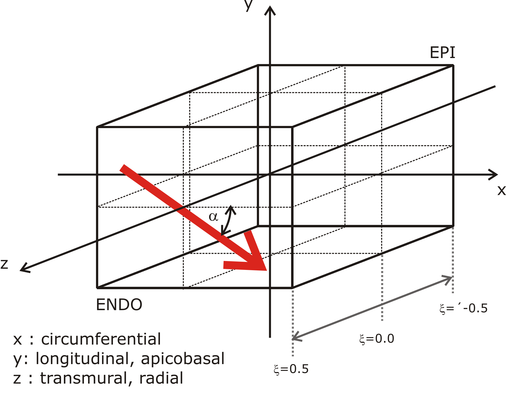
Note that the material coordinates in meshes generated by Block are as
illustrated below. Specifically, the  direction corresponds to the
circumferential direction,
direction corresponds to the
circumferential direction,  corresponds to the apical-basal direction
and
corresponds to the apical-basal direction
and  corresponds to the epi- to endocardium direction.
The other 3D mesh classes take the fibre_rule argument to the constructor,
which should be a function returning a helix angle in radians when passed a
normalised transmural distance (where 0 corresponds to endocardium and 1
corresponds to epicardium):
def rule(t):
    """
    +1 radian endo to -1 radian epi
    """
    return 1 - 2*t

# Or as a one-liner
rule = lambda t: 1 - 2*t

# Then to create a ring with this fibre rule
geom = mesh.Ring(5, fibre_rule=rule)

# Or even more compact
geom = mesh.Ring(5, fibre_rule=lambda t: 1 - 2*t)
The meshing code provides a convenience method for the generation of linear fibre rule in degrees or radians. For example, to generate the common +60 to -60 degree rule:
p60m60 = mesh.linear_fibre_rule(60, -60)
geom = mesh.Ring(5, fibre_rule=p60m60)
The 1D cable mesh always has a constant fibre direction aligned with the cable,
while the 2D grid mesh has a constant fibre direction assigned with the
fibres argument.
Tagging Regions
Block meshes can be tagged using one of three classes:
- An axis-aligned box (
carputils.mesh.BoxRegion) - A sphere (
carputils.mesh.SphereRegion) - A cylinder (
carputils.mesh.CylinderRegion)
See the class documentation for details on the exact arguments they take. They
all, however, take the tag argument, which specifies the tag to be assigned
to the elements inside the region:
geom = mesh.Block(size=(2,2,2))
reg = mesh.BoxRegion((-1,-1,-1), (1,1,0), tag=10)
geom.add_region(reg)
The other classes have tag regions assigned by passing a python function which returns True/False indicating whether a passed point is inside. For example, to assign a tag region to all points for positive x:
geom = mesh.Ring(5)
reg = lambda coord: coord[0] >= 0.0
geom.add_region(2, reg)
Note that the region tag must be passed separately in this case. The region
classes above can also be passed, however note that the tag defined in the
region object’s constructor is ignored in favour of that passed to
add_region.
Boundary Conditions
An additional convenience function
block_boundary_condition() is included to provide for the
easy definition of boundary conditions in block meshes. It uses the size and
resolution information from the geometry object to compute a box that surrounds
only the nodes of interest, and returns a set of CARP command line options. For
example, to define a stimulus on the upper-x side of a block:
geom = mesh.Block(size=(2,2,2))
bc = mesh.block_boundary_condition(geom, 'stimulus', 0, 'x', False)
The other mesh classes do not have an equivalent method, however the other 3D mesh classes offer functionality for the automatic generation of .surf, .neubc and .vtx files corresponding to relevant surfaces on the geometry. For example, with a ring geometry, you may wish to define Dirichlet boundary conditions on the top and bottom of the Ring and Neumann boundary conditions to the inner face. To generate files for these:
geom = mesh.Ring(5)
meshname = 'mesh/ring'
geom.generate_carp(meshname, faces=['inside', 'top', 'bottom'])
Which will generate files named like mesh/ring_inside.neubc.
Constraining Free Body Motion
You may also wish to take advantage of the generate_carp_rigid_dbc method,
which generates two vertex files for the purposes of preventing free body
rotation of the mesh. As illustrated in the image below, this includes two
points on the x axis and one on the y axis on the inner surface of the ring or
ellipsoid shell.
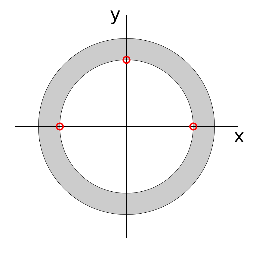
The files are generated by:
geom.generate_carp_rigid_dbc('mesh/ring')
which creates the files mesh/ring_xaxis.vtx and mesh/ring_yaxis.vtx. Dirichlet boundary conditions should be set up using these files, where the x axis nodes are fixed in their y coordinate and y axis node is fixed in its x coordinate. The first BC will then prevent free rotation and translation in the y direction, and the second will prevent translation in the x direction.
Implementation Details
Tessellation
An important consideration when generating a mesh in a subclass is how the resulting elements are to be tessellated into tetrahedra, which is done for most practical meshes used with CARP. Code to procedurally generate meshes in subclasses of Mesh3D generally use a combination of prisms and hexahedra to fill the geometry, however care must be taken to ensure that the edges of neighbouring elements match after the tessellation into tetrahedra is performed.
Hexahedra are deliberately tesselated in such a way that a grid of them which are all oriented in the same way will join up well when tessellated. There are two types of prisms available, offering the two possible ways for a prism to be tessellated.
When writing new mesh classes, the following nets provide a guide to the way in which these elements are tessellated. Printing these out and constructing the shapes aids considerably in figuring out how the elements mesh together.

Face Selection
The above nets also label each face. These are used in the mesh classes when generating elements to select particular faces for inclusion in generated surface and vertex files, which are themselves used for setting up boundary conditions in CARP simulations.
The _register_face method of the Mesh3D-derived classes is the way that
faces in the mesh are accumulated:
etype = 'hexa'
face  = 'front'
surface = 'endo'
self._register_face(etype, face, surface)
This will add the front face of the last hexahedron added to the mesh to the
endo surface. It is also possible to pass an exact element index to this
function, which by default just adds the last element of that type that was
added to the mesh.
Model Component Classes
The carputils.model subpackage provides an array of Python classes for
the set of CARP simulations in an object-oriented manner. Instead of manually
generating long lists of command line options such as:
opts = ['-num_imp_regions',        1,
        '-imp_region[0].im',       'TT2',
        '-imp_region[0].num_IDs',  2,
        '-imp_region[0].ID[0]',    1,
        '-imp_region[0].ID[1]',    2,
        '-imp_region[0].im_param', 'GNa=14']
you can represent the model component with a class instance:
from carputils.model.ionic import TT2IonicModel
imp = TT2IonicModel([1, 2], GNa=14)
and generate the option list with a single function call:
from carputils.model import optionlist
opts = optionlist([imp])
Any number of model components of different types can be generated in a single
optionlist() call, providing flexibility of use in run script logic:
from carputils import model

imp = [model.ionic.TT2IonicModel([1, 2]),
       model.ionic.TT2IonicModel([3, 4], GNa=14)]
cond = [model.ConductivityRegion([1, 2], g_it=1.5)]

opts = model.optionlist(imp + cond)
Classes check that the parameters passed to them are valid, ensuring that any mistakes due to typographical errors etc. are caught before execution of the CARP executable.
Detail on the usage of the various model class types is given below.
Conductivity Regions
Conductivity regions, defined by the class
carputils.model.ConductivityRegion, or its alias
carputils.model.GRegion, take a list of material IDs, an optional name
for the region, and the intra- and extracellular conductivity for the tissue.
See the class documentation for
the specific parameter names. See also the classmethods for easy definition of
passive and isotropic conductivity regions.
Example:
from carputils import model
# Tags 1 and 2, default conductivities
cr1 = model.ConductivityRegion([1, 2], 'myo')
# Tag 3, increased intracellular longitudinal conductivity
cr2 = model.ConductivityRegion([3], 'fast', g_il=0.2)
# Tag 4, isotropic conductivity
cr3 = model.ConductivityRegion.isotropic([4], 'iso', cond=0.1)
Eikonal Regions
Eikonal regions are defined by the class carputils.model.EikonalRegion
or its alias carputils.model.EkRegion. Unlike other classes, it
accepts only a single ID, which is actually the index of an existing
conductivity region. Like conductivity regions, it also has
isotropic() and
passive() class method alternate
constructors.
Examples:
from carputils import model
# Conductivity region 0, default conduction velocity
ek1 = model.EikonalRegion(0, 'myo')
# Conductivity region 2, isotropic conduction velocity
ek2 = model.EikonalRegion.isotropic(2, 'iso', vel=0.3)
Electrical Stimuli
The class carputils.model.Stimulus defines a model stimulus. The user
is expected to provide the relevant keyword arguments when using the class
directly, for example to define a stimulus with ‘somefile’ as the vertex
file:
from carputils import model
stim = model.Stimulus('pacing', vtk_file='somefile')
The keyword arguments (like vtk_file above) correspond with the fields of the CARP command line structure (-stimulus[0].vtk_file in this case).
Additional class methods exist for conveniently setting up a ‘forced foot’
stimulus, whereby the activation times from an Eikonal simulation are used to
drive a reaction-Eikonal simulation of electrophysiology. See the
class documentation for more information.
Ionic Models
Like the conductivity regions, ionic models also take IDs and name
arguments, however each different model takes its own set of optional
parameters. The different available models, their allowed arguments and their
default parameters can be found in the documentation of the
carputils.model.ionic module.
Example:
from carputils import model
imp = model.ionic.TT2IonicModel([1, 2], 'myo', GNa=14)
Active Tension Models
The active tension models are a special case in that they are not models in their own right, but are actually plugins to the ionic models. Active tension models, which only take the model parameters as command line arguments, are assigned to an existing ionic model using its set_stress method:
from carputils import model
# Create an ionic model
imp = model.ionic.TT2IonicModel([1])
# Create an active tension model
act = model.activetension.TanhStress(Tpeak=150)
# Assign the active tension model to the ionic model
imp.set_stress(act)
Available active tension models and their allowed parameters can be found in
carputils.model.activetension.
Mechanics Material Models
Like ionic models, mechanics material models take IDs, name and model
parameters as their arguments. Available models and their allowed parameters
are detailed in carputils.model.mechanics.
Example:
from carputils import model
mat = model.mechanics.NeoHookeanMaterial([1, 2], c=50)
Running A Simulation In plain mode
Using CARPentry
In this section the basic usage of the main executable CARPentry is explained. More detailed background referring to the individual physics electrophysiology, elasticity and hemodynamics are given below in the respective sections.
Getting Help
As in any real in vivo or ex vivo experiment there is a large number of parameters that have to be set and tracked. In in silico experiments tend to be even higher since not only the measurement setup must be configured, but also the organ itself. The general purpose design of carpentry renders feasible the configuration of a wide range of experimental conditions. Consequently, the number of supported parameters is large, depending on the specific flavor on the order of a few hundreds of parameters that can be used for experimental descriptions. With such a larger number of parameters it is therefore key to be able to retrieve easily more detailed explanations of meaning and intended use of all parameters.
A list of all available command line parameters is obtained by
carpentry +Help

carpentry [+Default | +F file | +Help topic | +Doc] [+Save file]
Default allocation: Global

Parameters:
         -iout_idx_file RFile
         -eout_idx_file RFile
         -output_level Int
         -num_emission_dbc Int
         -num_illum_dbc Int
         -CV_coupling Short
         -num_cavities Int
         -num_mechanic_nbc Int
         -num_mechanic_dbc Int
         -mesh_statistics Flag
         -save_permute Flag
         -save_mapping Flag
         -mapping_mode Short
         ...
         -rt_lib String
         '-external_imp[Int]' String
         -external_imp '{ num_external_imp x String }'
         -num_external_imp Int
and help for a specific feature is queried by
carpentry +Help stimulus[0].strength

stimulus[0].strength:
        stimulus strength

        type:   Float
        default:(Float)(0.)
        units:  uA/cm^2(2D current), uA/cm^3(3D current), or mV
        Depends on: {
                stimulus[PrMelem1]
        }
More verbose explanation of command line parameters is obtained by using the +Doc parameter
which prints the same output as +Help, but provides in addition more details on each individual parameter:
carpentry +Doc

iout_idx_file:
        path to file containing intracellular indices to output

        type:   RFile
        default:(RFile)("")


eout_idx_file:
        path to file containing extracellular indices to output

        type:   RFile
        default:(RFile)("")


output_level:
        Level of terminal output; 0 is minimal output

        type:   Int
        default:(Int)(1)
        min:    (Int)(0)
        max:    (Int)(10)


num_emission_dbc:
        Number of optical Dirichlet boundary conditions

        type:   Int
        default:(Int)(0)
        min:    (Int)(0)
        max:    (Int)(2)
        Changes the allocation of: {
                emission_dbc
                emission_dbc[PrMelem1].bctype
                emission_dbc[PrMelem1].geometry
                emission_dbc[PrMelem1].ctr_def
                emission_dbc[PrMelem1].zd
                emission_dbc[PrMelem1].yd
                emission_dbc[PrMelem1].xd
                emission_dbc[PrMelem1].z0
                emission_dbc[PrMelem1].y0
                emission_dbc[PrMelem1].x0
                emission_dbc[PrMelem1].strength
                emission_dbc[PrMelem1].dump_nodes
                emission_dbc[PrMelem1].vtx_file
                emission_dbc[PrMelem1].name
        }
        Influences the value of: {
                emission_dbc
        }
Details on the executable and the main features it was compiled with are queried by
carpentry -revision

svn revision:             2974
svn path:                 https://carpentry.medunigraz.at/carp-dcse-pt/branches/mechanics/CARP
dependency svn revisions: PT_C=338,elasticity=336,eikonal=111
Basic Experiment Definition
Various types of experiments are supported by carpentry. A list of experimental modes is obtained by
carpentry +Help experiment
yielding the following list:
| Value | Description |
|---|---|
| 0 | NORMAL RUN (default) |
| 1 | Output FEM matrices only |
| 2 | Laplace solve |
| 3 | Build model only |
| 4 | Post-processing only |
| 5 | Unloading (compute stress-free reference configation) |
| 6 | Eikonal solve (compute activation sequence only) |
| 7 | Apply deformation |
| 8 | memory test (obsolete?) |
A representation of the tissue or organ to be modelled must be provided in the form of a finite element mesh that adheres to the primitive carpentry mesh format. The duration of activity to be simulated is chosen by -tend which is specified in milli-seconds. Specifying these minimum number of parameters already suffices to launch a basic simulation
carpentry -meshname slab -tend 100
Due to the lack of any electrical stimulus this experiment only models electrophysiology in quiescent tissue and, in most cases, such an experiment will be of very limited interest. However, carpentry is designed based on the notion that any user should be able to run a simple simulation by providing a minimum of parameters. This was achieved by using the input parser prm through which reasonable default settings for all parameters must be provided and inter-dependency of parameters and potential inconsistencies are caught immediately when launching a simulation. This concept makes it straight forward to define an initial experiment easily and implement then step-by-step incremental refinements until the desired experimental conditions are all matched.
Picking a Model and Discretization Scheme
carpentry +Help bidomain
# explain operator splitting, mass lumping,
The time stepping for the parabolic PDE is chosen with -parab_solv. There are three options available.
Picking a Solver
The carpentry solver infrastructure relies largely on preconditioners and solvers made available through PETSc. However, in many cases there are alternative solvers available implemented in the parallel toolbox (PT). Whenever PT alternatives are available we typically prefer PT for several reasons:
- Algorithms underlying PT are developed by our collaborators, thus it is easier to ask for specific modifications/improvements, if needed
- PT is optimized for strong scalability, in many cases we achieve better performance with lightweight PT solvers then with PETSc solvers. In general, PT needs more iteration, but each iteration is cheaper.
- PT is fully GPU enabled.
Switching between PETSc/PT solvers is achieved with
PETSc solvers can be configured by feeding in option files at the command line. These option files are passed in using the following command line arguments
| ellip_options_file parab_options_file purk_options_file |
There are three options available.
After selecting a solver, for each physical problem convergence criteria are chosen and the maximum number of allowed iterations can be defined.
Configuring IO
TBA
Post-Processing Mode
Quantities appearing directly as variables in the equations being solved are directly solved for during a simulation. Other quantities which are indirectly derived from the primal variables can also be computed on the fly during a simulation, or, alternatively, subsequent to a simulation in a post-processing steps. On the fly computation is often warranted for derived quantities such as the instant of activation when high temporal resolution is important. For many derived parameters this may not be the case and it may be more convenient then to compute these quantities in a post-processing step from the output data. The computation of such auxiliary quantities such as, for instance, the electrocardiogram is available as postprocessing options. The post-processing mode is triggered by selecting
carpentry -experiment 4 -simID experiment_S1_2_3
In this case, the simulation run is not repeated,
but the output of the experiment specified with the simID option is read in
and the sought after quantities are computed.
Output of data computed in post-processing mode is written to a subdirectory
of the original simulation output directory.
The data files in the output directory of the simulations are opened for reading,
but other than that are left unchanged.
A directory name can be passed in with ppID. If no directory name is specified
the default name POST_PROC will be used.